Laboratory study and predictive modeling for thaw subsidence in deep permafrost

ZhaoHui Joey Yang,Gabriel T.Pierce

University of Alaska Anchorage,Anchorage,Alaska,USA

ABSTRACT Oil wells on the North Slope of Alaska pass through deep deposits of permafrost.The heat transferred during their opera‐tion causes localized thawing,resulting in ground subsidence adjacent to the well casings.This subsidence has a damaging effect,causing the casings to compress,deform,and potentially fail.This paper presents the results of a laboratory study of the thaw consolidation strain of deep permafrost and its predictive modeling.Tests were performed to determine strains due to thaw and post‐thaw loading,as well as soil index properties.Results,together with data from an earlier testing pro‐gram,were used to produce empirical models for predicting strains and ground subsidence.Four distinct strain cases were analyzed with three models by multiple regression analyses,and the best‐fitting model was selected for each case.Models were further compared in a ground subsidence prediction using a shared subsurface profile.Laboratory results indicate that strains due to thaw and post‐thaw testing in deep core permafrost are insensitive to depth and are more strongly influ‐enced by stress redistributions and the presence of ice lenses and inclusions.Modeling results show that the most statisti‐cally valid and useful models were those constructed using moisture content,porosity,and degree of saturation.The appli‐cability of these models was validated by comparison with results from Finite Element modeling.

Keywords:deep permafrost;thaw consolidation strain;predictive models;multiple regression analysis

1 Introduction

Oil wells in Alaska's North Slope pass through ap‐proximately 600 m of permafrost(Brown,1970;USGS,1993).The heat loss in production and injec‐tion wells during operation warms the adjacent perma‐frost around the well casing,causing the soil to thaw and subside over time.This subsidence has a damag‐ing effect,causing well casings to compress,deform,and potentially fail(Smith and Clegg,1971;Good‐man,1977,1978;Smith,1983;Yanget al.,2020).The consequences of such a failure can be severe.Ⅰt is thus desirable in the design and planning of new wells to be able to predict the magnitude of subsidence over a given period.

The engineering properties of permafrost,includ‐ing thaw strain,are closely related to its formation type and geologic history.Based on formation histo‐ry,permafrost can be generally classified as epigene‐tic,syngenetic,or polygenetic.Epigenetic perma‐frost forms when existing soil deposits are frozen in a later,cooler period.Many thousands or even mil‐lions of years can pass between deposition and freez‐ing(French and Shur,2010).Ⅰn many cases,epigene‐tic permafrost has had the time and necessary condi‐tions to consolidate prior to freezing.On the other hand,syngenetic permafrost forms through a rise of the permafrost table in a cold climate during the de‐position of additional sediment or other earth materi‐al.Under these conditions,the soil is often frozen before it can densify or consolidate.Due to their dif‐ferent geneses,thawing epigenetic permafrost typi‐cally results in smaller settlements than syngenetic permafrost.On the North Slope of Alaska,the perma‐frost is polygenetic,i.e.,a combination of both for‐mation types,with its upper regions composed of layers of syngenetic permafrost and its lower regions consisting of epigenetic formations(French and Shur,2010).

Ⅰn the case of oil wells in permafrost,thawing is a localized phenomenon with a specific type of geome‐try.For instance,oil flows through production wells to the surface at temperatures between 60 and 85°C(Palmer,1972).Heat transfer to the surrounding permafrost creates a localized,cone‐shaped region of thaw,commonly referred to as a thaw bulb,cen‐tered about a long,cylindrical well.The radius of the fully‐thawed zone,RTB,increases in size over time as the thaw front advances away from the well casing laterally in all directions.According to thermal modeling for an oil field on the Alaska North slope(Matthewset al.,2015),the rate ofRTBincrease varies with thermal properties and initial conditions and de‐creases with time,and single well models predicted that the averageRTBreaches 2.4−3.2 m in 5 years and 3.6−6.0 m in 20 years.

The soil within a thaw bulb does not always bear the full weight of the overlying soil column due to arching effects.Arching is a form of stress redistribu‐tion that occurs due to shear stresses at boundaries be‐tween yielding soils and unyielding masses(Terzaghi,1943).Ⅰn thaw bulbs,these boundaries include the well casing or casing insulation,and the surrounding frozen soil.At both boundaries,laterally‐transmitted shear stresses bear some of the burden.According to Palmer(1972),arching is generally ineffective to a depth of approximately 5RTB.At greater depths,arch‐ing effects become significant and can provide most of the support(Mathewset al.,2015;Yanget al.,2020).

Very limited work is available for thaw strain pre‐diction of shallow permafrost.Crory(1973)outlined a method for predicting thaw settlement in a soil layer based only on an initial frozen dry unit weight and an assumed final thawed dry unit weight.This method depends solely on dry unit weights and is theoretical‐ly valid for all soil types provided they are fully satu‐rated.Another method was developed by Nelsonet al.(1983)by employing an empirical equation developed from statistical analysis of sample data.Thaw consoli‐dation tests were performed on 1,024 samples taken from boreholes that spanned the centerline of the en‐tire 1,300‐km‐long Trans‐Alaska Pipeline.The sam‐ples were grouped into nine distinct classes according to the unified soil classification system(USCS),and a multiple regression analysis was performed for each soil class using porosityn,moisture contentω,and degree of saturationSas the independent variables.The empirical model proposed by Nelsonet al.(1983)has the advantage of accounting for partially‐saturat‐ed soils and ice lenses by including the independent variablesSandω.However,this model was construct‐ed on tests of samples recovered from depths of 15 m or less,making its broader applicability to deeper de‐posits an unknown.Neither model made a distinc‐tion between strains due to thaw and those due to post‐thaw loading.Studies of thaw characteristics of deeper permafrost do not exist based on the authors'knowledge.

This study attempts to fill the gap on thaw strains of deep permafrost and aims to develop empirical methods based on laboratory testing data for predict‐ing ground settlement due to thaw of deep permafrost.Laboratory testing program and a summary of index and thaw consolidation test results are presented first.Several predictive models and their statistical parame‐ters are presented for thaw consolidation at various conditions.The best models for individual cases are selected and are applied to a study site,and the ground subsidence predictions are compared with that from a rigorous computer simulation.Key assump‐tions and limitations are also addressed.

2 Laboratory testing program and results

As part of a project aiming to study the thaw sub‐sidence of oil wells drilled through deep permafrost,five boreholes aligned on a cross‐section at a study site in the Alaska North Slope were advanced to as deep as 166 m using a sonic drilling method to extract continuous,minimally disturbed permafrost cores of 10 cm in diameter.Selected samples from all five boreholes were tested to provide various material properties for thermal and mechanical modeling(EBA,2013;Matthewset al.,2015;Zhanget al.,2017a,b;Wanget al.,2019;Yanget al.,2020).Exten‐sive thaw consolidation tests were conducted for thaw subsidence modeling.Details regarding the thaw‐consolidation test cell,loading system,speci‐men preparation,and loading procedure can be found in EBA(2013)and Pierce(2019),and only a summary is provided below.

The custom‐designed thaw consolidation test cell has an inner diameter of 6.35 cm and a height of 12.7 cm.Figure 1 shows the major components and their dimensions.Two identical cells were fabricated to allow for quick interchange between sequential tests.The initial frozen cores were reduced to a diame‐ter of 6.3 cm inside a cold room set at−10°C.This re‐sizing was performed by rough‐cutting by band saw and fine‐machining by lathe,such that the specimen could slide into the testing cell with no discernable space between the soil and the cell wall.

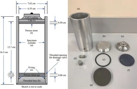
Figure 1 Sketch of the custom cell for frozen core thaw consolidation testing,showing:(a)specimen cylinder;(b)threaded base;(c)cell loading cap;(d)drainage control;(e)rubber O‐ring;(f)upper porous stone;and(g)lower porous stone

Thaw and post‐thaw were considered to be two sep‐arate phases of the thaw consolidation test(EBA,2013).Strains measured in the lab can be broken into two separate categories:thaw strain,εT,and post‐thaw consolidation,εC,where consolidation is applied in the broader sense that includes effects due to both densifi‐cation and the expulsion of pore water.The sum ofεTandεCis the total strain,εTC.The thaw phase was per‐formed with drainage restricted over a 24‐hour period,which was confirmed as an adequate time for the com‐plete thaw to take place at an ambient temperature of 22°C.The post‐thaw phase was conducted immediate‐ly after the thaw phase,and the drainage was opened to allow for the consolidation of saturated or mostly‐satu‐rated specimens.Each step was allowed to continue un‐til the specimen height had leveled off with time.

Specimens were loaded in multiple steps in which the pressure applied was a certain percentage of the total overburden pressure,σvwhich was determined by the depth of the sample and the average density correlated with depth.The percentages selected were based on the testing phase and the depth range of the sample,and the scenario corresponding to the thaw bulb withRTB=7.5 m was assumed based on the cur‐rent status in the study site.A conservative approach was taken in determining the maximum overburden stress to apply for a given depth range during the thaw phase.The threshold depth used to differentiate between shallow and deep specimens was 30 m(Yanget al.,2020).Ⅰn the shallow range,even though the vertical stress ratio decreases almost linearly with depth from the ground surface,it was decided to ig‐nore possible stress redistributions and apply 100%ofσv.After thaw,the specimens were unloaded in two 10‐minute steps to 60%and 20%σvfor post‐thaw phase testing.Ⅰn the deep range,the maximum stress was selected as 20%σv.The loading schedule for the consolidation phase includes loading and unloading with the maximum overburden stress to 130%ofσv.

Ⅰndex property tests were performed for each sam‐ple and were conducted either on the thaw consolida‐tion specimen after test completion or on the trim‐mings saved during specimen preparation.Each sam‐ple was tested for its gravimetric moisture content(ASTM D2216‐10,2010),density(ASTM D7263‐09,2009),gradation(ASTM D422‐63,2007),and pore water salinity(by conductivity instrument).For in‐stance,Table 1 presents the index properties of speci‐mens from borehole 2M obtained at the University of Alaska Anchorage(UAA).Moisture contents ranged from 6.8%to 163%,with a mean of 29%.Each grada‐tion test included analyses by both sieve and hydrome‐ter due to the high fines content in all samples,and soils were predominantly poorly‐graded or gap‐grad‐ed.Figure 2 displays the particle size distributions for three representative soil samples.Only five of the samples tested were deemed non‐plastic,and the rest were tested for Atterberg limits(ASTM4318‐17,2017).All samples were formally classified according to the USCS(ASTM D2487‐11,2011).After classifi‐cation,six representative samples were selected for specific gravity tests(ASTM D854‐14,2014).

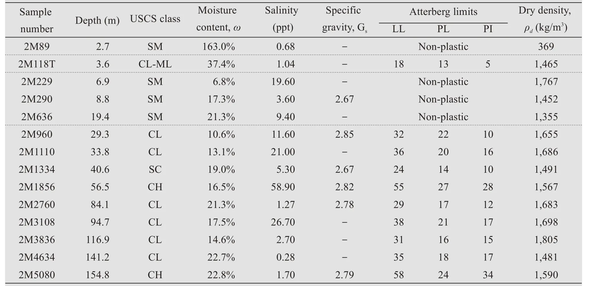
Table 1 Summary of index properties and classifications of permafrost samples from borehole 2M

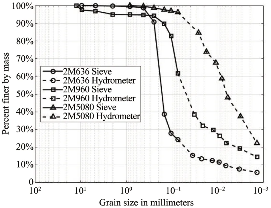
Figure 2 Grain‐size distributions for selected samples by sieve and hydrometer analyses

Testing data from a total of 12 thaw consolidation specimens(labels beginning with 2M)obtained at UAA were supplemented by the data reported in EBA(2013)for predictive modeling.Table 2 lists the com‐bined dataset with thaw consolidation test results and index properties.Methods adopted in the UAA labora‐tory program were designed to be comparable to those performed in EBA(2013)so that the results of both programs would be compatible.Combining both data sets increased the potential sample size from 12 to 33.Overall,the porosities of the tested data used for modeling vary between 0.336 and 0.515,the mois‐ture content values fall in between 6.8%and 37.3%.Note that soil types from the EBA testing listed in Ta‐ble 2 only include USCS classifications for sandy soils,which were based on particle size analysis,and silts and clays were not formally classified and are listed simply as"Fine".

3 Predictive modeling

The laboratory testing program carried out in this study combined with that of EBA(2013)provide a da‐tabase for predictive modeling of thaw settlement of deep permafrost.This section describes the multiple regression models and their statistical performances,a comparison of the model predictions with laboratory test results,the optimum models for various scenari‐os,and the application of the final proposed models in an oil field.

3.1 Multiple regression models

A total of four cases were chosen for further analysis,and they include:(1)thaw strain at 20%σv,(2)total strain at 20%σv,(3)thaw strain at 100%σv,and(4)total strain at 100%σv.These four distinct cases were chosen to represent different phases and loading scenarios during thaw.Case 1 and Case 3 ex‐amined the strains due to thaw only,whereas Case 2 and Case 4 concerned cumulative strains that includ‐ed the effects of continued loading post‐thaw.Case 1 and Case 2 combined all available data for strains measured under loading at 20%overburden pres‐sure,corresponding to the in‐situ vertical stress con‐dition due to arching effects and stress redistribu‐tions within the thaw bulb.Cases 1 and 2 thus are the most applicable for predicting strains across a deep soil profile extending below 30 m.On the oth‐er hand,Case 3 and Case 4 combined all data for loading at 100%overburden pressure without consid‐eration of stress redistributions and are applicable for shallow permafrost and deep permafrost thaw bulb with a radius large enough to prevent stress redistribution.

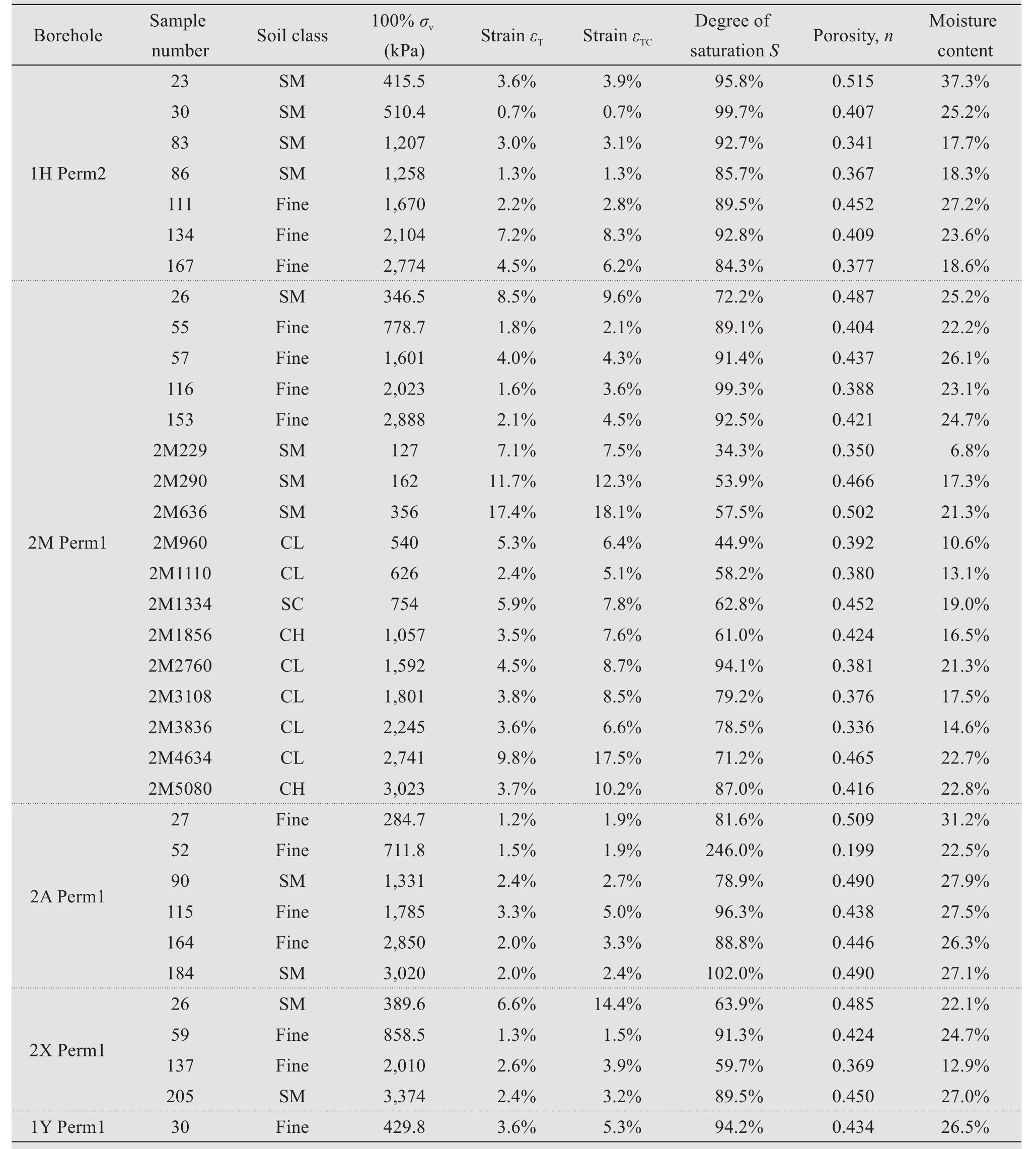
Table 2 Permafrost thaw consolidation testing data and their index properties

Several additional independent variables,includ‐ing depth,density(wet and dry),and visible ice con‐tent,were added to those(i.e.,porosity,n,degree of saturation,S,and gravimetric moisture content,ω)considered in Nelsonet al.(1983).The visible ice content is defined here as the percentage of observed ice recorded on the original sample core logs.Figure 3 depicts the variation of strains for Cases 2 and 4 with depth,with the visible ice content shown for ref‐erence.While strain values were observed to general‐ly decrease with increasing depth,like that of visible ice content,the trend was slight.These new variables were found to provide little contribution and were therefore eliminated from further analysis.The use ofS,n,andωas parameters is also supported theoretical‐ly for their importance in relation to soil volume re‐duction during thaw(Andersland and Ladanyi,2004).As a result,the thaw consolidation data were com‐bined across all depths and all types of soils to per‐form statistical modeling for reasons including its lim‐ited size and unconsolidated nature of the syngenetic permafrost samples.

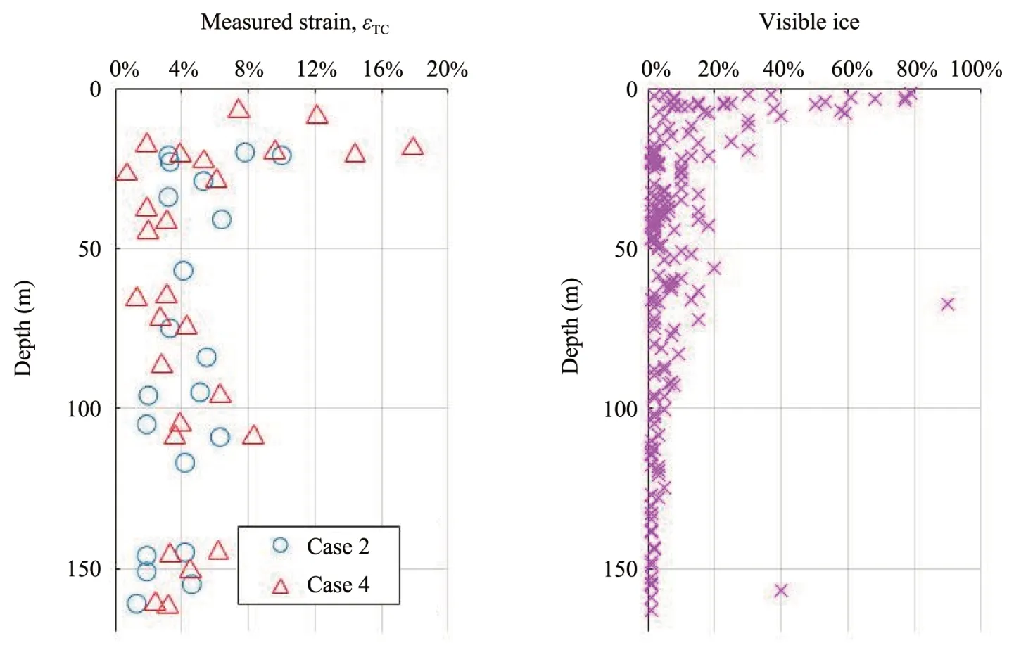
Figure 3 Comparison between measured strains and observations of visible ice content for Cases 2(total strain at 20%σv)and 4(total strain at 100%σv)

The empirical equation(Equation(1))derived from shallow permafrost at depths of 15 m or less,to‐gether with the published regression coefficientsAiproposed by Nelsonet al.(1983),was first applied to the test data.

However,the predictions did not satisfactorily match the laboratory data,indicating Equation(1)is not directly applicable for deep permafrost.Nonethe‐less,it served as a starting point,and the development of models suitable for Cases 1 through 4 involved nu‐merous permutations.A total of three models were considered in this study.Two new models were devel‐oped from different combinations ofS,n,andω.These models are hereafter referred to as Model 1 and Model 2.Models 1 and 2 are given respectively as

whereεis the predicted strain,nthe porosity,ωgrav‐imetric moisture content,Sthe degree of saturation,andA0,…,Anregression coefficients that vary with the selected case.While early attempts to apply the model and regression coefficients by Nelsonet al.(1983)were unsuccessful,the general form of Equa‐tion(1)was used to re‐fit to the deep permafrost test data and designated as Model 3 in this study for comparison.

Multiple regression analyses were performed with these three statistical models on the laboratory data in the four cases identified previously.Table 3 summa‐rizes these statistics.The validity and utility of poten‐tial models were evaluated by an analysis of variance global test using theF‐statistic at theα=0.05 level of significance,and the overall predictive accuracy pro‐vided by the standard error of the regression,Se.The standard null and alternative hypotheses for determin‐ing model utility were applied here as:

Ho:All model terms are unimportant for predict‐ing strain values;

Ha:At least one model term is useful for predict‐ing strain values;

The rejection region was established from tablulat‐ed values forF＞FαwhereFαvalues for Cases 1 through 4 were 2.555,2.459,2.509 and 2.509,respec‐tively.Values of the multiple coefficient of determina‐tion,R2,and the adjusted multiple coefficient of deter‐minationR2

awere also considered.R2awas given more weight thanR2because it is more conservative and is unbiased by the relationship between the sample size and the number of parameters in the model(Mc‐Clave and Sincich,2000).The results of the globalF‐tests,along with the comparison plots with the labo‐ratory‐measured strains,show that each of the models provided an acceptable fit of the data for all four cas‐es.P‐value determinations resulted in the rejection of the null hypothesis for all three models.There was thus sufficient evidence to conclude that each model is statistically useful.Ⅰn terms of the standard error and the multiple coefficients of determination,the dif‐ferences between each model were minor.Figure 4 through 7 compare the predicted strains by all three models with the laboratory‐measured strains.While all three models were able to capture the general trend of the laboratory‐measured strains across the depths,careful examination between the predicted and labora‐tory‐measured strain values show the various perfor‐mance of these models in the four cases.

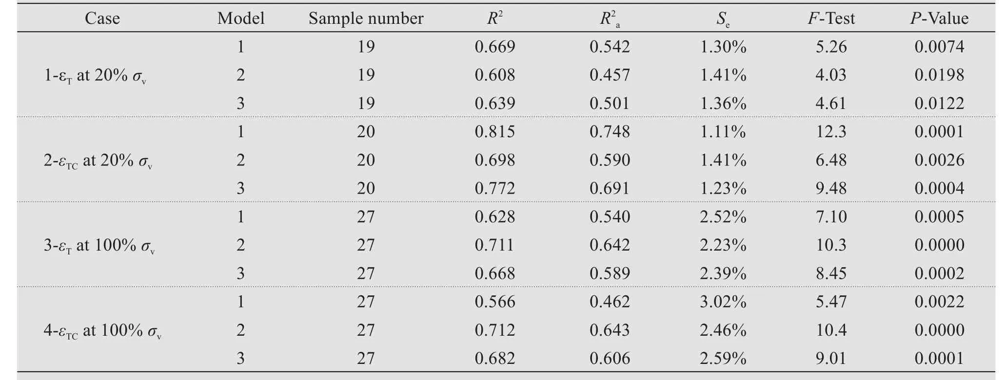
Table 3 Statistical summary for the three models applied to all four cases

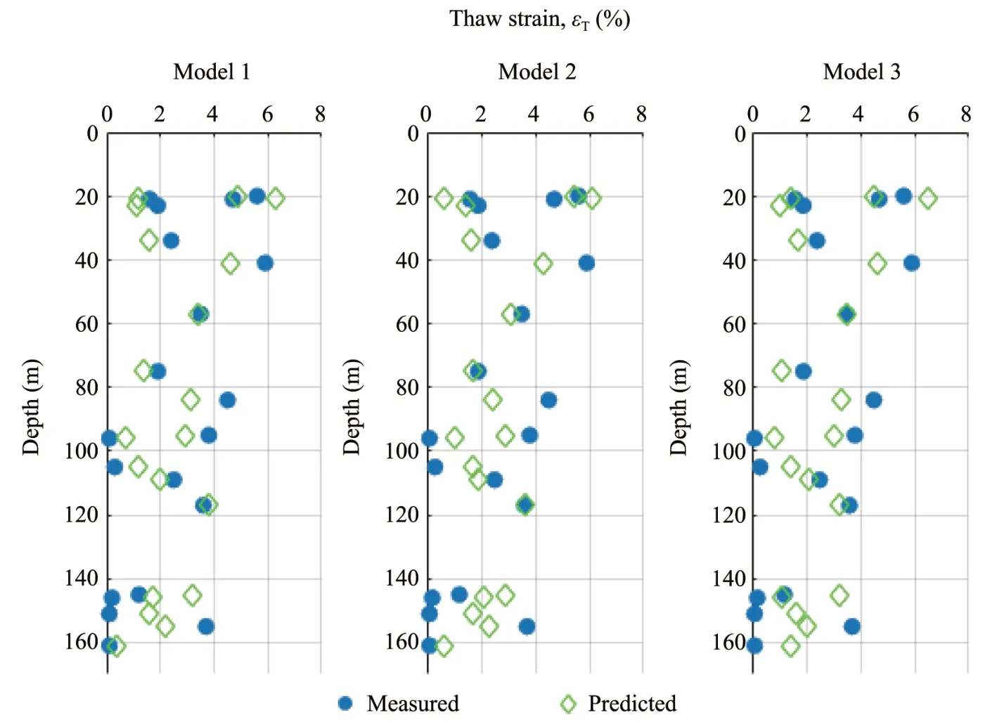
Figure 4 Thaw strain comparison for Case 1(20%σv)

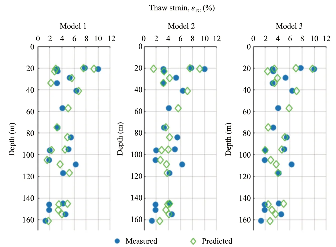
Figure 5 Total strain comparison for Case 2(20%σv)

Figure 6 Thaw strain comparison for Case 3(100%σv)

3.2 Selected models

Models providing the best statistical fit can be se‐lected based on the values in Table 3 and by compari‐son between the model predictions and laboratory da‐ta.Table 4 shows the best‐fitting model and its regres‐sion equation for each case.Each of these best‐fitting models had both the lowestSeand the highestas well as the lowestP‐value from the globalF‐test.The magnitudes of theP‐values and theF‐statistics were not compared between models during selection;the trend is merely noted.The best fit was provided by Model 1 for Cases 1 and 2,while Model 2 did so for Cases 3 and 4.Model 3 was neither the best nor the worst statistical fit for any one case.The standard error values for the best‐fitting models were less than 2.5%.Ⅰt is worth noting that,compared with those thaw‐strain empirical models presented in Andersland and Ladanyi(2004),the current models make use of a set of index properties(i.e.,S,nandw),instead of just one(e.g.,the frozen bulk density or total frozen soil water con‐tent)and had much less prediction error.Additionally,the thaw‐consolidtion models presented in Andersland and Ladanyi(2004)assumed that the frozen soil was saturated.Hence,they are not readily application for the tested samples,which are mostly unsaturated.

Figure 7 Total strain comparison for Case 4(100%σv)

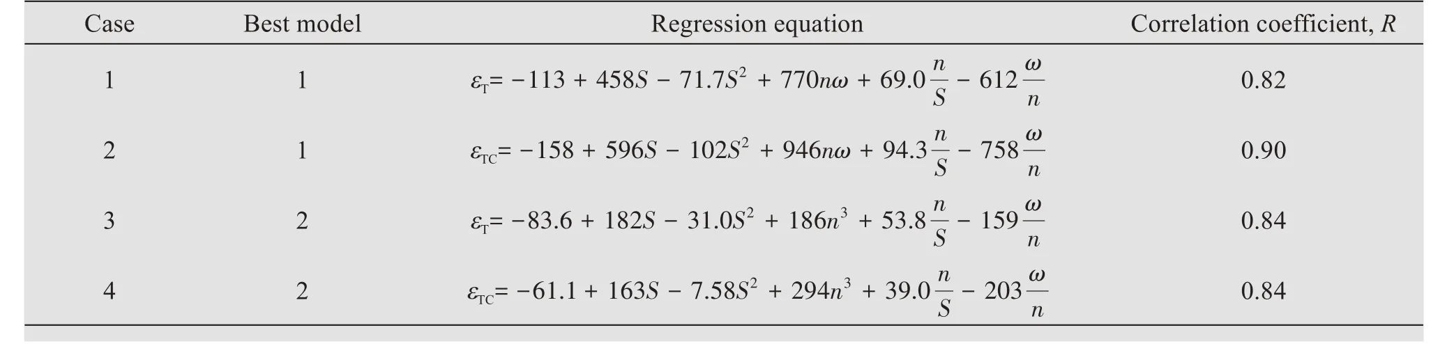
Table 4 Selected best regression model for each case

3.3 Model application

Application of these regression equations to a site and comparison of the model predictions with other independent analyses of ground subsidence help to validate these models.The single well case study by Yanget al.(2020)provides a field case for this purpose.Model 1,Model 2,and Model 3 were applied to the same permafrost stratum along with the index properties.Table 5 lists the ground surface subsidence predictions by all three models for the four cases,and Figures 6 and 7,as examples,display the variation of ground settlement with depth for Cases 2 and 4,respectively.As can be seen from Ta‐ble 5 and Figures 8 and 9,the results of the surface subsidence predictions varied widely yet consistent‐ly by model.Ⅰn all cases,magnitudes at a given depth increased in the order of Model 1,Model 2,and Model 3.While Model 3 had provided reason‐able fits of the strain data for each case,the subsid‐ence prediction for this particular subsurface profile was unreasonably high.

Since the overburden pressure varies with depth and the radius of the thaw bulb,neither of these four cases would be directly applicable to the field condi‐tions.Ⅰn fact,for the current conditions at the study site,i.e.,RTB=7.5 m after about 30 years of opera‐tion,the stratum at the top 30 m is equivalent to Case 2,while that below 30 m aligns better with Case 4.Therefore,using Model 1,the average of predictions from these two cases,i.e.,2.56 m,can be used as a reasonable ground subsidence prediction.Although no field survey data of ground subsidence is available for prediction,the predicted subsidence compares fa‐vorably with that from sophisticated Finite Element modeling by Yanget al.(2020),i.e.,2.70 m.

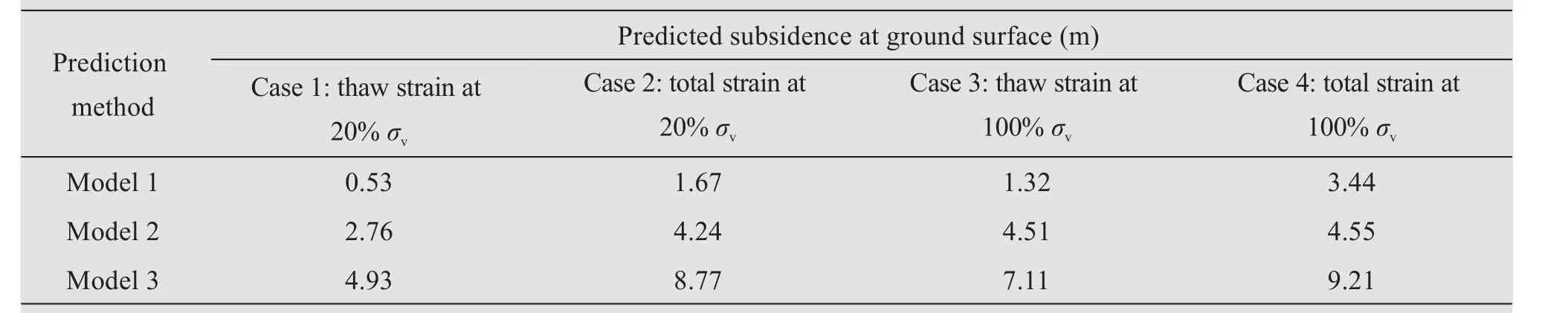
Table 5 Comparison of ground surface subsidence predictions

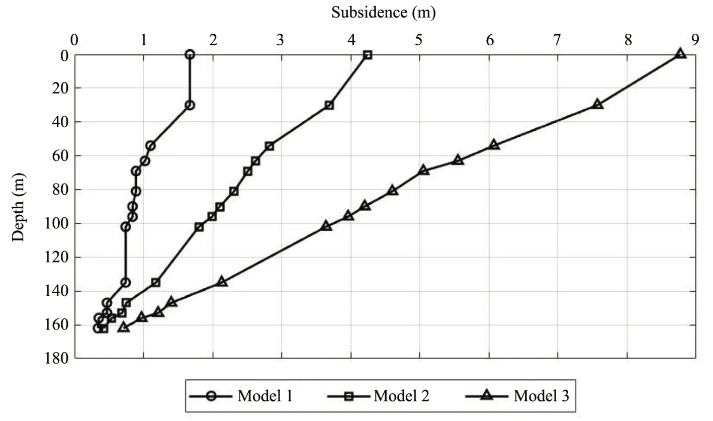
Figure 8 Subsidence predictions for Case 2(Total strain at 20%σv)

4 Discussions on limitations and assumptions

The regression models developed and used in this research were all applied to a very limited data set.While the overall sample size was greater than 30,not all data was available for every case analyzed,and the largest set contained 27 data points.The two main rea‐sons for having different numbers of data points for each case were:(1)many of the 20%σvstrain values from EBA(2013)were back‐calculated from displace‐ment vs.time graphs for samples tested at 100%σv,and several of these graphs were missing,and(2)the testing program developed at UAA applied a maxi‐mum of 20%σvto samples recovered from 30 m or greater.This decision was made during program de‐velopment prior to analysis work.

Simplifying assumptions were made in the recre‐ation of in situ stress conditions.These assumptions are reflected in each of the four cases analyzed.Cases 1 and 2 both account for the effects of stress redistri‐butions within the thaw bulb forRTB=7.5 m.Model‐ing results by Mathewset al.(2015)indicate that the time of formation of such a large thaw bulb exceeds 20 years.For time periods shorter than 20 years,the model will likely tend to overpredict subsidence magnitudes.Cases 3 and 4 do not consider stress re‐distributions at all and,therefore,limited to applica‐tions at shallow depths or for the thaw bulb that is large enough to prevent arching effects and stress redistribution.

5 Conclusions

A comprehensive testing program was carried out to evaluate the thaw consolidation strains of deep permafrost sampled from the North Slope of Alaska.These testing results,together with data from a previous study,were used to develop predic‐tive models.The sample index properties were test‐ed and reported.A custom‐designed thaw consolida‐tion test cell and the testing procedure were de‐scribed in detail.The thaw consolidation strain data was presented,and three multiple regression models were compared to select best‐fit models for various cases considering stress redistribution due to arching effects during the thaw of permafrost around an arc‐tic oil well.The following conclusions can be drawn from this research:

(1)While strain values were observed to decrease with increasing depth,like that of visible ice content,the trend was slight.This observation shows the im‐portance of cryostructure over depth for unconsolidat‐ed syngenetic permafrost formations.

(2)Empirical models using terms formed from the variables S,n,and were the only ones analyzed that provided reasonable fits of the measured strain data.Depth,density,and overburden pressure were found to provide no direct value as independent variables in any regression iteration attempted.

(3)Model 1 provided the best statistical fit of the measured strain data for the conditions given by Case 1 and Case 2,while Model 2 provided the best fit for Case 3 and Case 4.Model 3 was neither the best nor the worst fit for any of the four strain data cases.

(4)These best‐fit models were validated by com‐parison of the predicted surface subsidence with so‐phisticated Finite Element modeling results for an arc‐tic oil well.

Moisture content,wet bulk density,and specific gravity are the only properties that need to be deter‐mined before the application of either of these models in strain predictions for a permafrost stratum.These properties and the soil profile data can all be obtained from the results of a typical geotechnical exploration and laboratory testing program.One should be cau‐tious when applying these models with input parame‐ters outside of the ranges of this data set.

Acknowledgments:

The authors gratefully acknowledge the permafrost core donation by ConocoPhillips Alaska to the Uni‐versity of Alaska Anchorage,which made the labora‐tory study possible.