Tuning of active disturbance rejection control for differentially flat systems under an ultimate boundedness analysis: a unified integer‑fractional approach

Jeisson E. Otero‑Leal · John Cortés‑Romero · Efredy Delgado Aguilera · Felipe Galarza‑Jimenez ·Alexander Jimenez‑Triana

Abstract

Keywords ADRC · Fractional-order system · Ultimate bound · Final value theorem

1 Introduction

The feedback control theory has been developed under different paradigms throughout the years. There are two wellestablished tendencies: on one hand, we have the modelbased control (modern control), and on the other hand, we have the error-based empirical design paradigm. These two ideas have taken a divergent development from each other,with the scholars and many researchers preferring the first one given its strong mathematical background.

The control strategies under the model control paradigm,although new and constantly evolving, often present several challenges and problems at the time of implementation. One of this problems-among others-is the uncertainty in the model of the system used for the design, which frequently does not fully represent it. Moreover, many disturbances have uncharacterized magnitudes and even nature.

This problem is also reflected in many publications involving practical experimentation of the different control techniques, where no details of the experimentation are given, nor a guide of how to exactly reproduce the results taking into account the possible problems in every stage of the process. One of the most common pieces of missing information is the tuning values of the parameters of controllers, which are usually found after a sometimes long and tedious process, as well may know every practitioner.The problem of tuning parameters is often disregarded by scholars in opposite of what one may see in industrial applications, where these values are of central interest. As consequence, a variety of auto-tuning or ad-hoc algorithms have been proposed for control of industrial processes reflecting a lack of technical knowledge and comprehension of the problem, and hence, it seems necessary further research on a tuning process with strong mathematical background and simple enough to be applied to the daily needs of practitioners.

As a middle ground between these two techniques, the active disturbance rejection control (ADRC) is presented as an alternative. ADRC has been emerging as a new trend for control of linear and non-linear uncertain systems under the influence of unknown external disturbances. Under this approach, exogenous disturbance along with uncertainty parameter and non-modeled dynamics are considered as an equivalent-input-disturbance. This disturbance can be estimated in a linear context where a reduced linear control uses an online estimation for a proper tracking task [1]. Typically,ADRC is considered in the context of differentially flat systems using extended-state observer-based control schemes for trajectory tracking problems. This methodology is fundamentally linear rendering a simplified but efficient approach.

The acceptance of this technique has been growing in the later years, mainly for its application on systems with uncertainties. One of the most valuable idea of ADRC is the treatment of the non-linear systems as perturbed linear systems, this idea has allowed to propose different approaches to specific cases and system structures. Other recent works address the topic of the differential order of the differential equation used to model the system. Extensive literature covers fractional-order systems or to be more precise, fractional-order control systems, of which the integer order is considered as a particular case of study. Hence, the study of fractional-order control systems provides a unified framework for the analysis.

The advantages offered by the ADRC control technique can be properly used within the context of fractional-order control. Particularly, the intrinsic reduction to a perturbed linear simplified system of commensurate order can reduce the stability analysis to the characterization of the influence of the equivalent disturbance on this system. This work presents an extension of the ADRC methodology to differential fractional-order (linear and non-linear) systems based on simplified perturbed linear systems of commensurate order.

Most of the proposed analyses, for both integer and fractional differential order, hold the stability as the most relevant requirement for the design of control systems [2-4].Thus, these works develop a stability evaluation using modern theory for fractional-order systems [5, 6]. In the linear case, the Matignon criterion established an imperative reference [7], and some other analyses have derived from this result [8]. For a certain class of integer- and fractional-order systems, the results in [9] and [10] reported a Lyapunov-like stability analysis respectively.

The goal of this work is to show the practical benefits of the ADRC technique in comparison with well-established controllers in the industry such as PID and similar methods.Usually, there are no clear and practical guides for tuning both controller and observer, and this gap in knowledge is even bigger in the study of systems with uncertainties. It is convenient to derive a standardized tuning process with a strong mathematical support which guarantees a set of performance indices. The performance of the control system can be evaluated through indices that consider mainly steady-state tracking and estimation errors. This work is an extension of the results reported in [11], and attempts to establish this practical standardized tuning process for the ADRC technique.

The scheme here proposed is composed of two stages.The first stage relies on setting a desired bandwidth for the frequency response of the closed-loop system which will allow us to set a first set of values for the parameters of the controller and the observer. This step guarantees the stability of the closed-loop system but not necessarily the desired performance and it is widely describe in the literature [12].The second stage and main contribution of this work is a fine-tuning of the observer parameters. This fine-tuning guarantees a maximum error of the unified disturbance signal estimation and, given the structure of the system, it also guarantees a maximum error for the other state estimations which are used in a linear control law. All this is granted via an ultimate boundedness analysis. This analysis is summarized in some formulas relating the ultimate bounds of the estimation and tracking error with the parameters to be tuned.

Using the bandwidth of the observer as a tuning parameter has been already applied in ADRC [13], and its properties analyzed in [14]. The authors in [15] propose a tuning process when the plant is known and show the improvement of the performance in comparison to the bandwidth method. In [16], biological algorithms are implemented to tune the parameters, and in [17], a linear matrix inequalitybased method is proposed. A uniform ultimate bound for the tracking and observer error is found in [18]; additionally,some conditions on the parameters are offered to guarantee stability of the closed-loop system, although it does not offer an explicit guide for the tuning of these parameters, since their main contribution is other.

The present work exhibits the following content. A rigorous mathematical analysis concludes with the establishment relations between the estimation and tracking errors and the control and observer parameters.

The proposed analysis of the boundedness of the tracking and estimation errors allows to propose a guideline for tuning the observer-based control system parameters under the ADRC approach. Finally, a natural extension of a fractionalorder system analysis to an integer-order system analysis offers a wider applicability of the results useful for stability analysis purposes.

The remainder of this paper is organized as follows.Section 2 presents the derivation of the model and the proposed control law. In Sect. 3, the main result is presented,where the ultimate estimation error is upper bounded by an expression containing explicitly the tuning parameters.Additionally, it is shown how to apply this result in a tuning algorithm. Section 4 deals with the relation between the observer estimation error and the tracking error. In Sect. 5, it is offered a numerical example. Finally, Sect. 6 summarizes the accomplishments of this work.

2 Model and control law

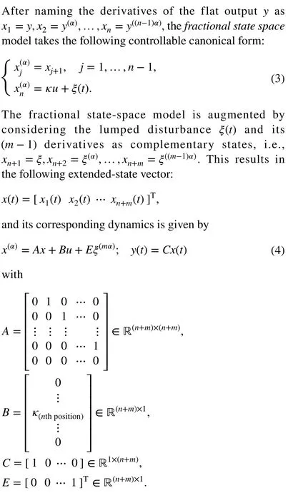
In this section, we present a detailed derivation of the socalled linear system with lumped disturbances and a control law whose tuning is the central matter of this work. For a flat-output fractional-order non-linear plant with equivalent input disturbances, the proposed fractional-order ADRC(FOADRC) approach consists of i) an augmented fractionalorder state-space model; ii) a fractional-order GPI observer employing the concept of a fractional-order extended-state observer [19]; and iii) an observer-based control law to solve the trajectory tracking problem.

2.1 Dynamic system modeling

Consider a disturbed non-linear scalar fractional-order differentially flat system represented by the following function with commensurate orderαand 0＜α≤1:

whereκis thecontrol input gainof the system, the termφ(·) is addressed as thedrift function, andζ(t) represents the external disturbances (see Appendix A for definitions and important previous results on fractional-order dynamical systems). The drift function takes into account the remainder linear or non-linear dynamics. The unperturbed system,namely whenζ(t)=0 , is the aforementioned differentially flat system expressed as a function of fractional derivatives of the flat outputy(t) [20].

The additive linear and non-linear dynamics expressed inφ(·) are uncertain due to: (a) the lack of knowledge of certain parameters, (b) the presence of unmodeled statedependent non-linearities, or (c) the combination of these two previous cases with the presence of uncertain exogenous time-varying disturbances signals. Therefore, it is convenient and without any lost of information to consider all those terms as a single, lumped, unstructured, time-varying disturbance termξ(t) [21]. This allows simultaneous, though approximate, state and lumped disturbance estimation regardless of any particular internal structure. As a result,the following simplified system can be defined:

where the signalξ(t) can be considered as the sum ofζ(t)andφ(·).

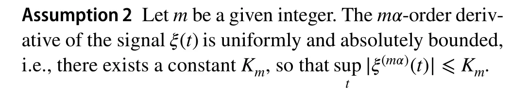
Regarding the system (2), the following assumption is made:

Assumption 1 The disturbance functionξ(t) is completely unknown, while a reasonable knowledge of the control input gainκis granted.

Remark 1Assumption 1 takes into account the fact that the magnitude order of the signals involved in the system and the controller operation are known, thus strong knowledge of the scaling factor is provided for the control input signal.The performance of this system modeling is highly dependent on the estimation quality ofξ(t) . Therefore, it is necessary to implement a generic internal model of the unified signal. This internal model is appended to a simplified linear plant model to produce an augmented model.

2.2 Augmented fractional state‑space model

2.3 Fractional‑order GPI observer‑based approach

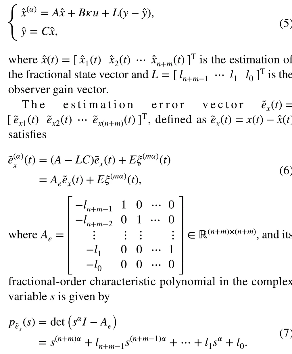
The fractional-order generalized proportional integral observer (FGPI observer) takes the structure of a classic Luenberger observer, which consists in a copy of the augmented system complemented by weighted injections of the output estimation error,1=y-:

Assumption 3 All the eigenvalues ofAeare defined to be negative real numbers.

Remark 4The simplified model proposed in this work needs this bound due to the uncertainties in the internal model of the system and the disturbance. It is also important to notice that if the disturbance possesses high-frequency components, multiple derivatives of these specific components will derive in higher bounds needed for the signal.

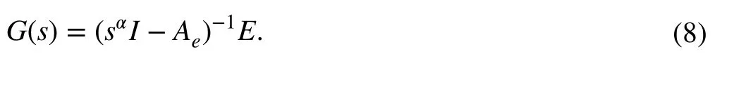
It is possible to find a vector estimation transfer functionG(s), by defining the state estimation error vector as the system output and the signalξ(mα)(t) as the input of the system:

2.4 FGPI observer‑based control law

In the previous section, the relationship between the performance of the fractional-order observer and the observer gains was proved. Moreover, if the observer gains are high enough,the closed-loop system under the FGPI observer-based control strategy ensures the reference tracking error to a small vicinity of zero.

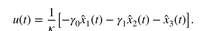
Therefore, consider the next control inputu:

whereuLis an effective fractional control law conditioned to given specifications, andis the estimated value of the unmodeled perturbation defined in (2). Inspired by a minimum realization approach and ensuring the maximum use of the estimations provided by the observer, the following FGPI observer-based control is proposed to establish a dominant error tracking dynamics:withγn=1.

Lemma 1The disturbance rejection output feedback controller(10)drives the trajectory of the controlled system output error ey(t)toward a desirable vicinity of zero,when the set of coefficients{γ0,…,γn-1}is properly chosen.

ProofThe equation in (11) has a fundamental solution for the left part of the equality defined by the characteristic polynomialpcthat is designed to have its roots in the stable region. The right part of the equation is a function of.The last section proved that everyis bounded; therefore,the right part is seen as the response of a stable system to a bounded signal input.

Albeit the solution of the right-hand term of (11) is unknown, it has a bound that depends on the coefficients of the observer and the outer feedback controller, therefore,the tracking error can be reduced to a desirable vicinity of zero. ◻

Remark 5Given a good performance of the FGPI observer,the right part of (11) becomes rapidly small, allowing the linear dominance of the left-hand term to follow the dynamics of the tracking error. In practice, if the settling time of the estimation errors is configured to be at least three times faster than the settling of tracking error, observer and controller can be designed independently.

Another version of the control law requires an additional step in the formulation of the simplified dynamic system presented in Sect. 2.1. The main idea is to take into account the tracking error instead of the state variables. This procedure facilitates the observer-based control law, eliminating the need of multiple derivatives of the reference signal used to form the error polynomial.

Hence, starting with (2), the next operation is made:

This controller structure provides an easier way to implement the algorithm taking advantage of the estimation of the variablesxjthat already represent an error. It is assumed that every error should go to zero; therefore, the reference is zero.

3 Main result

So far, it has been proposed a control law based on the FGPI observer. However, from (11), it is concluded that the correct estimation of the states and the disturbance signal is key for this strategy, since the tracking error dynamics depend on the estimation errors.

3.1 Ultimate boundedness analysis

The purpose of this section is to provide analytic expressions for the ultimate bound of each estimation error. It results interesting that each bound can be very close to the maximum value of the estimation error.

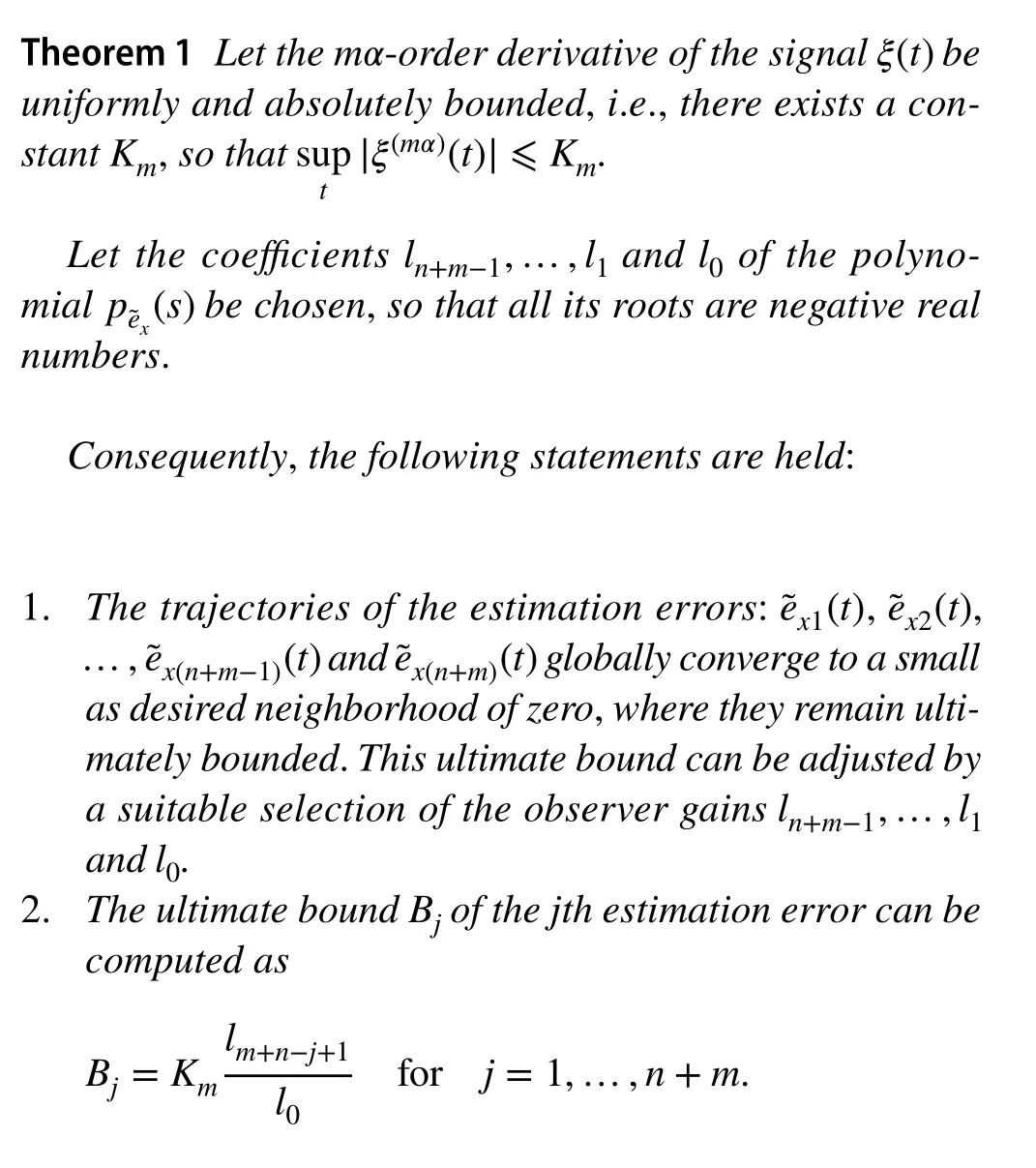
According to this theorem, when the steady state is achieved, each estimation errorexiis not greater than the given boundBj. This result can be used in the observer tuning process as it will be shown later. For now, the proof is presented.

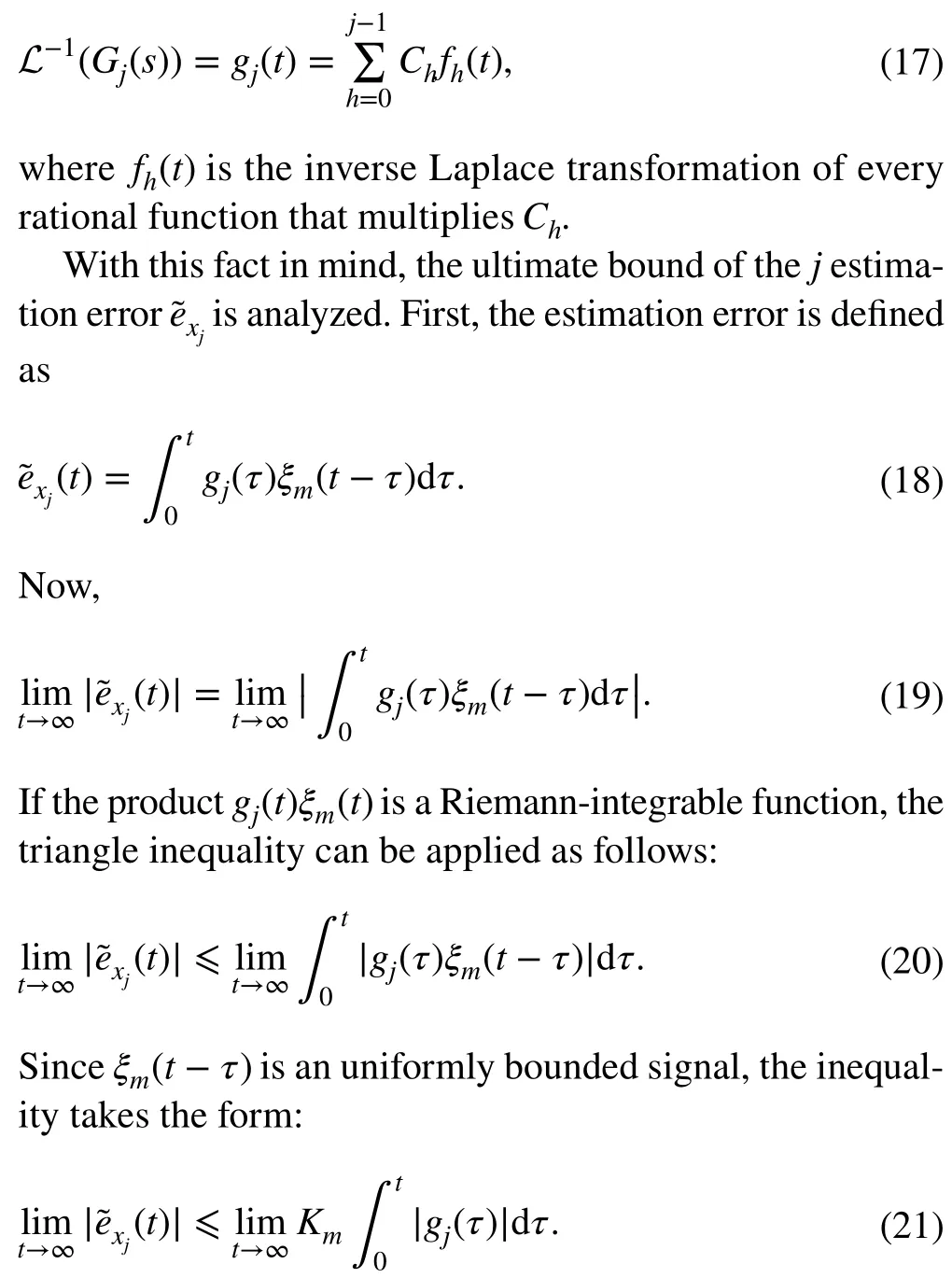
ProofThe problem is addressed by analyzing independently the convergence of the estimation errors related to the new virtual inputξ(mα)(t) . Without loss of generality, one of these rational functions is taken and decomposed in a series of factors that explicitly displays the roots of the function. Under the proper conditions of positiveness of the functions, the ultimate boundedness analysis determines the expected constant bound related to the observer gains.

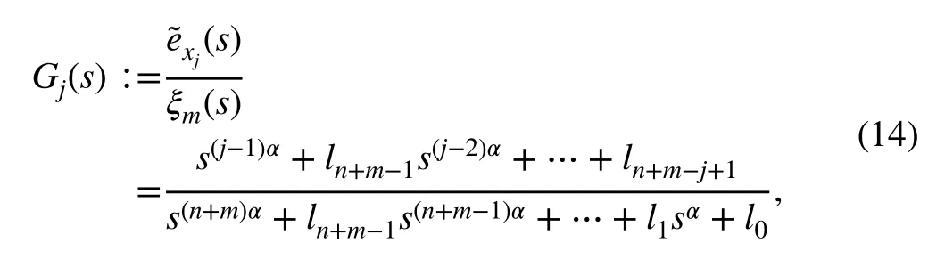
To analyze the extended-state estimation errors in time domain, the transfer functionG(s) is used to compute the Laplace transform of each estimation error.G(s) is composed of the transfer functionsGj(s) with 1 ≤j≤n+m.These functions take into account the effect of the disturbanceξ(mα)(t) on each estimation error and have the following form:

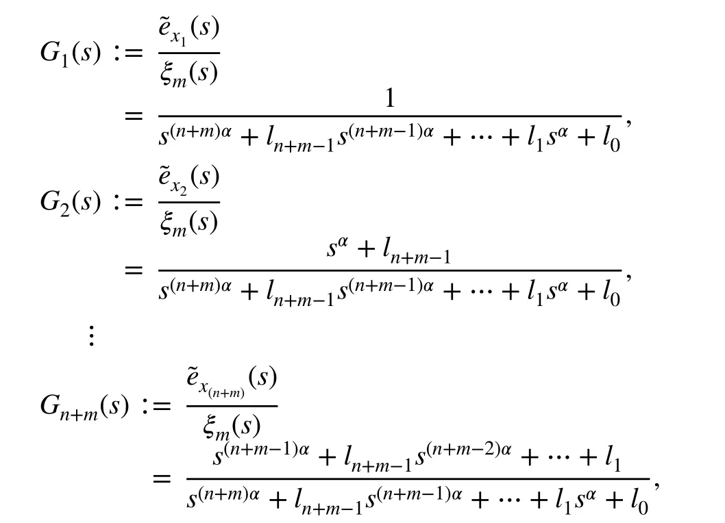
whereξm(s) representsξ(mα)(t) . It can be seen that all the components ofG(s) have the same denominator corresponding to the characteristic polynomial of the observer. This polynomial depends on the design parametersln+m-1,…,l0that are determined by the selection of the poles.

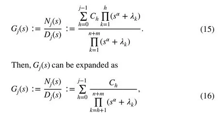
Considering the transfer function:

and the result described in Appendix B,Gj(s) can be written as follows:

TheGj(s) transfer function written in the time domain has the form:

Given the corresponding structure ofGj(s) , it is possible to prove thatgj(t)≥0 fort≥0 . Refer to Appendix B for the details of this proof.

Thus, the last expression (21) may be written as follows:

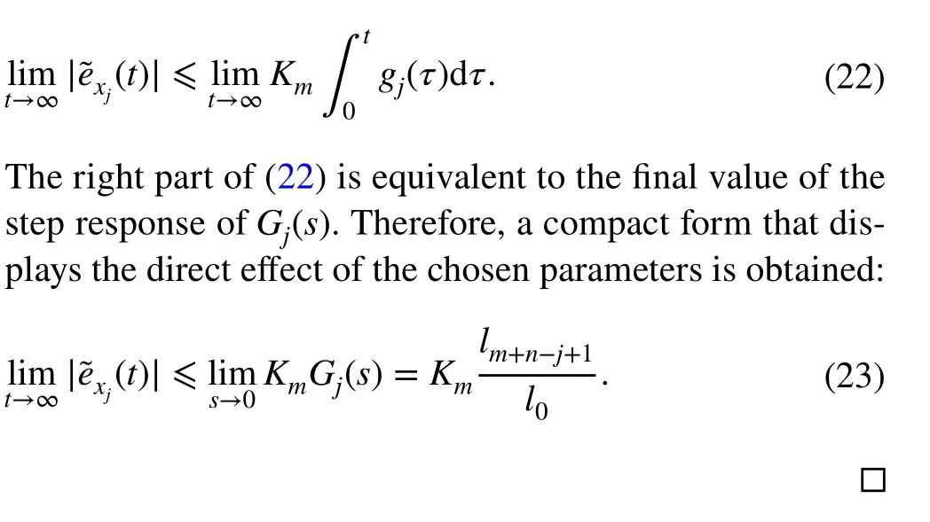
Given that the disturbance bound is unknown in most cases, it is not possible to use directly (23) to determine the bound of the estimation errors. Even if the first estimation error is known, it is not possible to know what is the value of the bound predicted by (23) for this error. However, as it will be explained below, the bounds given by (23) are equal to the maximum value of the estimation errors if the bandwidth of the observer is large enough.

3.2 Maximum value of the estimation errors for a large bandwidth observer

If the bandwidth of the observer is much larger than the disturbance bandwidth, the transient ofgi(t) is faster than the disturbance. Recall thatgi(t) is the impulse response of each transfer functions that were designed to be stable; therefore,their responses will fade in time. In addition, the lumped disturbance contains the internal dynamics of the system and the external disturbances that, without loss of generality, are assumed bounded, but not convergent to zero.

Considering this, the convolution integral describing the evolution of the system in time can be approximated by computing the integral just to a finite value oftclosed to the settling time ofgj(t) , hereafter calledT. The expression relating the estimation error develops as follows:

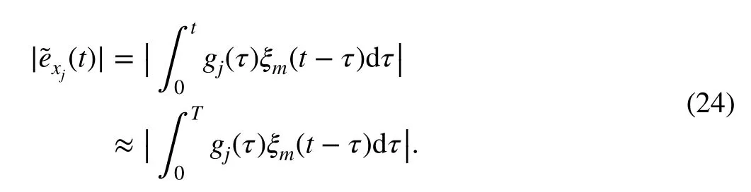
IfTis small enough,ξm(t-τ)≈ξm(t) in the integration interval:

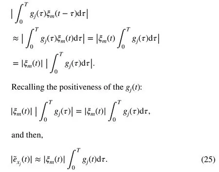
The last expression implies that the maximum value of the estimation error is approximated by the value of the ultimate bound.

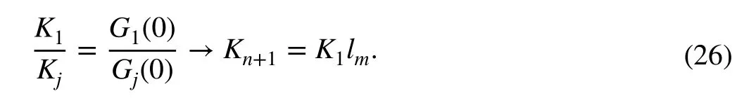
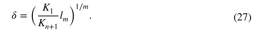
This result allows to conclude that it is possible to compute the bound of the disturbance estimation errorKn+1from the output estimation errorK1. Under the aforementioned conditions, these bounds are equal to the maximum value of the estimation error, leading to the following expression:

3.3 Algorithm for the observer tuning

The following algorithm summarizes sufficient conditions for stability and good performance of the observer-based control law. The idea is to offer a guided iterative process for the tuning of the observer parameters which is key to achieve the control.

1. Establish a bound for the disturbance estimation error,which under these conditions is the same maximum value.

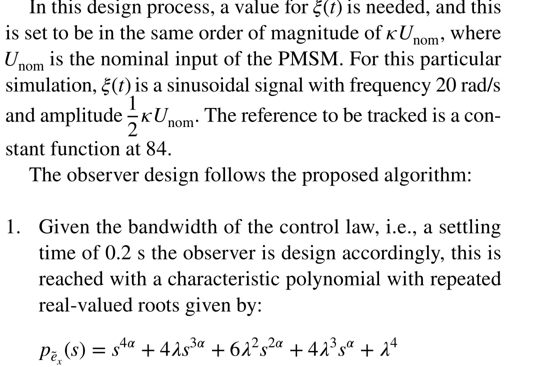
2. Place the poles of the observer using the information about the bandwidth of the plant and the external disturbances. This process can be carried out by the identification of the frequency and gain scales of the plant and the application of the procedure described in [12].As general rule, the bandwidth of the observer is chosen to be larger than bandwidth of the plant and the disturbances.

3. Amplify the roots of the characteristic polynomial of the estimation error by a factor (δ ＞1 ). The new characteristic polynomial takes the following form:

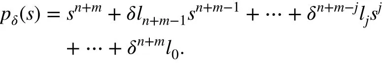
Multiplying by just one factor is done for the sake of notation and brevity of the equations, but the applicability of the result is not reduced to this case. After the first adjustment, measure the output estimation error.

4. If the new output estimation error isδn+mtimes smaller than the first one, then the conditions are fulfilled and the procedure can continue. Otherwise, increase the amplification factor until the conditions are guaranteed.

5. Let us suppose that the condition of the previous step is fulfilled. In this stage, it is possible to measure the output estimation error and take its maximum value asK1. According to (26), it is possible to compute the last amplification factorδto achieve the desired value ofKn+1for the disturbance estimation. In fact, it is given by:

6. Applyδto every root of the characteristic polynomial of the estimation error.

4 Influence of the estimation error on the tracking error

According to (11), the tracking error dynamic is related to the estimation error as follows:

deriving an upper bound for the tracking error.

5 Closed‑loop stability analysis

In this section, BIBO stability of the closed-loop system is proved. Taking into account that the input of the closedloop system is the reference, let us suppose that this signal is bounded. Now, it is required to prove that the output of the system is bounded, as well.

According to the analysis shown in the previous section and in (29), the tracking error is bounded as follows:

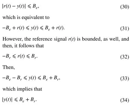
Thus, the output signal is bounded as required.

6 Numerical example

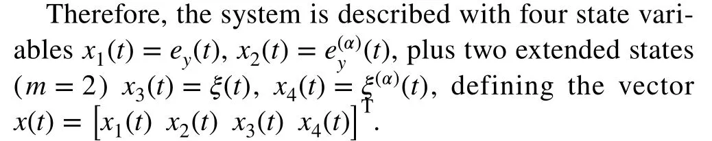
This section shows the control design process and some simulation results for a permanent magnets synchronous motor(PMSM) whose two models were validated by experimental data in [23] were the velocity is the output to control. Similar procedures for the control of an induction motor and a brushless DC motor can be found in [24, 25], respectively. The design of the controller is based on the integer-order model,as shown in (35), and the fractional-order version in (36).The results here presented validate the control-law design algorithm in Sect. 3.3 also reflecting the unified aspect of the ADRC methodology for integer- and fractional-order systems. Additional to the controller, a saturation block for the control signal is added to represent a feeding voltage limitation of ±200 V:For each model, a controller is proposed and validated following the proposed design algorithm for a sinusoidal disturbance and a constant reference.

On one hand, the fractional-order model in (36) is clearly incommensurate and it is taken as the plant to validate the performance of the controllers (each one designed for different models as it will be illustrated ahead). Throughout the design process, it will be shown that its incommensurate order generates no further complications. On the other hand, the integer-order model presents the challenge of choosing a fractional order for the controller to obtain similar performance to what it is shown in [23]. It is important to clarify that the goal of this numerical example isnotto analyze and compare the performance of the each plant model nor the closed-loop system, but to exemplify the design methodology in Sect. 3.3 and how this is independent from the differential order of the plant and controller.

The simulations are made on MATLAB/Simulink, with a fixed-step of 0.0001 s, and the solver ODE4 (Runge-Kutta).This is the support for the library FONCOM which contains blocks for fractional-order operations. These are set for a frequency range of 0.001-1000 rad, and an approximation of 5.

6.1 FGPI design for fractional‑order system

For a better visualization of whereU(s) andξ(s) are, the equationGfr(s) is reorganized as follows:

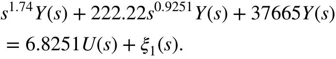
The tracking error is defined asey(t)=y(t)-y*(t) which will be the output of the system. After subtractings1.74Y*(s) on both sides, it system results in

withκ=6.8251 , andξ(t) being the lumped disturbance as defined in (12).

The design process starts taking the system in (37) and finding a suitable commensurate order for it. As the literature shows, it is recommended to take the this order closed to 1, which for this caseα=1.74∕2=0.87 results in a appropriate value [11].

Now, the observer of extended states takes the form in(5), and the estimations given by it are used in the construction of a control law according to (9) which results in

The bandwidth of the systems is determined by fixing repeated real roots at -40 , i.e.,γ0=1600 ,γ1=80 , which translates to a settling time around 0.2 s as also shown in the experimental results in [23].

withλ=66.

2. Withλ=66 , the value ofK1is 1.65. If theλ=2×66 ,the expected value ofK1is 0.1031 (=1.65∕16 ), but the resulted value is 0.55 instead, which means that the bandwidth that guarantees the results of this work regarding the ultimate bounds is not yet reached.

3. It is setλ=10×66 , resulting inK1=1.545e-3 . To check the bandwidth condition, it is setλ=2×10×66 gettingK1=9.55e-5 ≈1545e-3∕16 which is the expected value. This means that the bandwidth condition is met.

4. The desired ultimate bound for the estimation error is 0.01% , i.e.,K3=317 . Using theλ=660 , the scaling factor in (27) is computed, gettingδ=1.77.

5. With these values for the observer, the ultimate bound for the tracking error is computed as in (29):

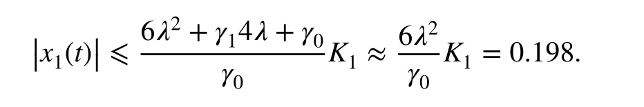
Hence, the roots of the characteristic polynomial of the observer are at -660 . Figure 1 displays the results of the simulation. It can be verified that in the stationary state,its magnitudes are scaled by 6λ2, and that the maximum value in steady state for the tracking error is 0.16. Additionally, the control signal saturates for the first 7 ms,which is according to the characteristic initial overshoot for the extended-state implementation of ADRC [26].

6.2 FGPI design for integer‑order system

In this case, the modelGint(s) is given in (35), and it can be reshape as follows:

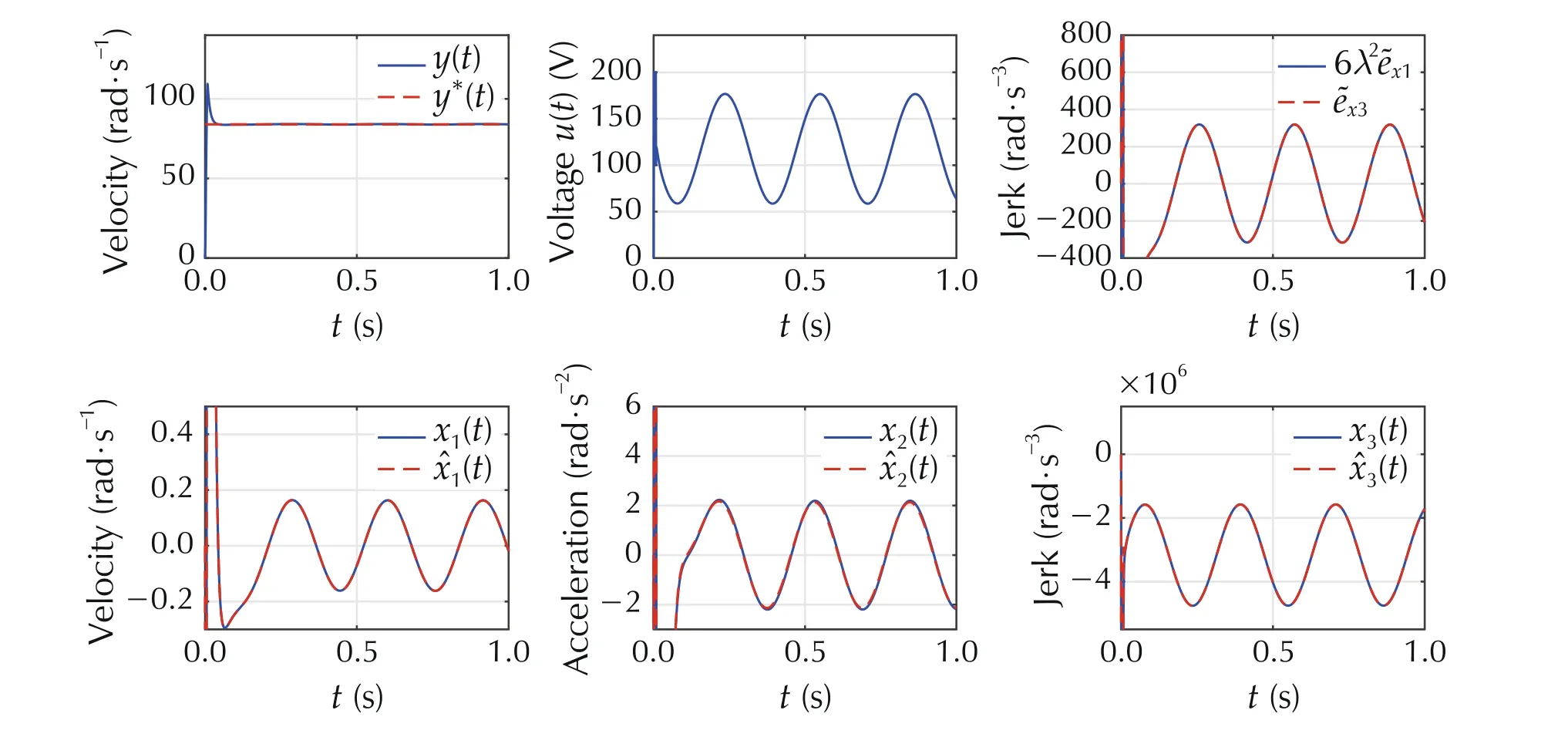
Fig. 1 Tracking, control, estimates, and estimates errors for fractional design

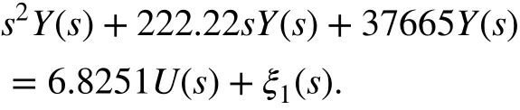
As before, the tracking error is given byey(t)=y(t)-y*(t)and it is also the output of the control law, and hence,s2Y*(s)is subtracted on both sides, resulting in:

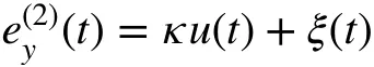
withκ=6.8251 . The constant reference to track is 84 rad/s.From this point, the characterization and the desired control law are the same that ones made for the fractional-order case and are skipped.

The observer design follows the proposed algorithm:

Since this process is the same as before, fewer comments are given.

1. It is setλ=66 for the characteristic polynomial of the estimation error.

2. Withλ=66 ,K1=1.65 and withλ=2×66 ,K1=0.57 and not 0.1031 that is the expected value if the bandwidth conditions are met.

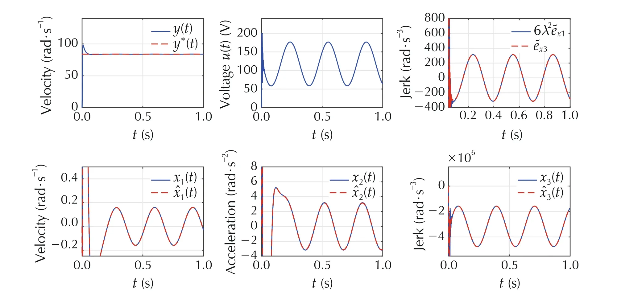
Fig. 2 Tracking, control, estimates, and estimates errors for integer design

3. In the second iteration, it is setλ=10×66 , gettingK1=3.57e-3 , and forλ=2×10×66 ,K1=2.12e-4 ≈3.57e-3∕16 as expected.

4. The desired ultimate bound for the estimation error is again set at 0.01% , i.e.,K3=317 . Usingλ=10×66 ,the scaling factor isδ=2.64 . Hence, the roots of the characteristic polynomial of the observer are at -660.

5. The ultimate bound for the tracking error is the same as before and the result in simulation is 0.16 of error. The simulations of the integer order are presented in Fig. 2.

It is important to notice that overshoot presented in the observer estimation in both simulations (see Figs. 1 and 2 )is a characteristic behavior of the high-gain extended-state observers [26]. In many situations, the magnitude of the overshoot requires the implementation of a “clutch” to introduce the estimation signal, so that it does not perturb the whole system [11]. However, this implementation is out of the scope of this work, since the goal is to show the bounded tracking error in steady state which behaves as expected.

It is concluded that the design and tuning procedure for the integer- and fractional-order case is the same. Given this model, the fine-tuning for each case is also similar(δint=2.64 ,δfr=1.77 ). This difference may be a result from the better performance of the fractional-order system in comparison to the integer-order one [23]. The observerbased control methods as ADRC may require a high gain which shows its disadvantages in the presence of noise.

7 Conclusions and future work

An effective adaptation of ADRC based on a simplified commensurate fractional-order model reference has been presented, obtaining a unified fractional- and integer-order modeling process and control law design. An stability analysis is proposed regarding the ultimate bound of the estimation and tracking errors. The result here presented provides a guideline for tuning the observer-based control-law parameters, offering a practical assistance in the implementation or simulation process.

Appendix A: concepts on fractional‑order systems

A generalization of the integer-order dynamic systems is found in fractional-order systems (FOS), providing better mathematical tools for the modeling of physical and engineering systems [22]. For this matter, it is necessary to give some definitions taken from the fractional calculus [27].

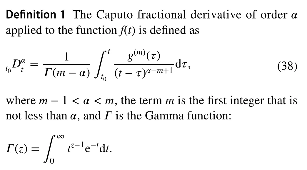
The Caputo fractional derivative is chosen, because its properties facilitates its application to dynamic systems [27].

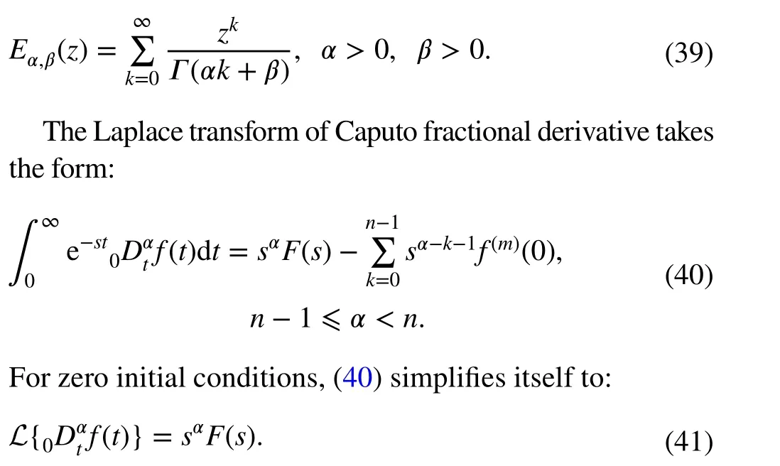
Definition 2 The two-parameter Mittag-Leffler function is defined as

For the sake of brevity, theα-order Caputo derivative for af(t) function will be represented asf(α)witht0=0 and 0＜α≤1.

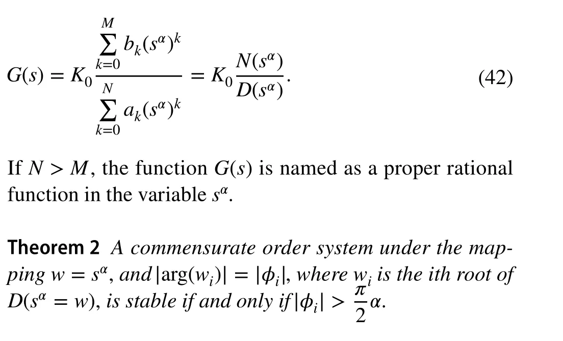
In the case of commensurate order systems, the transfer function takes the following form:

According to [28], the final value theorem (FVT) is applicable under stability conditions, even when there is a branch point ats=0 for a FOSf(t):

Appendix B: Proof of the positiveness of gj(t)

A fundamental aspect for the proof of Theorem 2 is the positiveness ofgj(t) , i.e.,gj(t)≥0 fort≥0 . The expression in (17)shows with ease that if every productCi fiis non-negative,gi(t)is also non-negative. Therefore, the cases for the functionfiand the constantCito be non-negative are shown.

Positiveness of fi

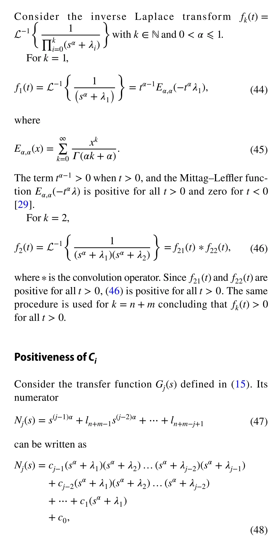
where the coefficientscj-kare given by

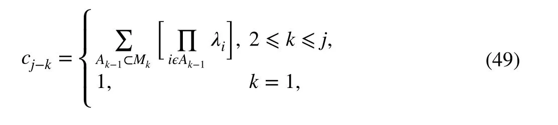
whereMk={j-k+2,j-k+3,j-k+4,…,n+m} andAk-1is ak-1 element subset ofMk, so the sum is made over allk-1 element subsets ofMk. Given that the Assumption 3 holds, all thecj-kare positive real numbers.

The proof of this is built by strong induction, matching the resultingcj-kcoefficients with the respective coefficientslkseen in (14).

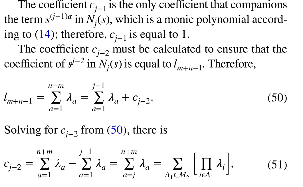
whereM2={j,j+1,j+2,…,n+m} andA1is a single element ofM2, resolving this waycj-2.

To proof the validity of (49) for the coefficientscj-kwithk ＞2 , suppose that is true for 2 ≤k≤k0-1 , and let prove it true fork0=k.

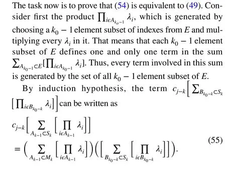
First, the coefficient ofsj-kin (48) is calculated and labeled asCresulting ink0-kelements from the set {j-k0+2,j-k0+3,…,j-k+1} , but this set has exactlyk0-kelements,so all its elements must belong toAk0-1. However, it is impossible, becauseAk0-1must havek0-kelements fromSk={1,2,3,…,j-k} , and this set excludes the elementj-k+1 . Therefore,Ak0-1does not belong toDk0-1, andAk0-1∈PE-Dk0-1. This implies that all the elements that belong toPMk0belong toPE-Dk0-1, and then,PMk0⊂PE-Dk0-1.

Consider now a setAk0-1which belongs toPE-Dk0-1,and suppose thatAk0-1∉PMk0. Then,Ak0-1includes at least one element from the set {1,2,3,…,j-k0+1} , butAk0-1does not belong toDk0-1. Now, suppose thatAk0-1includesl1elements from{1,2,3,…,j-k0+1} , and it includes all the elements from the set Ω={j-k0+l1+1,j-k0+l1+2,…,j-1} . In this case,Ak0-1hask0-1 elements fromS1={1,2,3,…,j-1} and no element fromM1,so it belongs toDk0-1, which is a contradiction. Therefore,Ak0-1must exclude at least one element from Ω . Suppose thatj-k0+l1+αis the first element in Ω , which is not included inAk0-1, ifα=1 ,Ak0-1hasl1elements fromSk0-l1andk0-1-l1elements fromMk0-l1, soAk0-1∈Dk0-1, and this is a contradiction. If 2 ≤α≤k0-l1-1 , thenAk0-1hasl1+α-2 elements fromSk0-l1-α+2andk0-l1-α+1 elements fromMk0-l1-α+2, soAk0-1∈Dk0-1which is another contradiction. Therefore, it is concluded thatAk0-1∈PMk0,and subsequentlyPE-Dk0-1⊂PMk0andPMk0=PE-Dk0-1,which is the expression in (56) that proves the validity of(54), and finishing the proof of (49) by strong induction.

withAk-1⊂Mk,Bk0-k ⊂Sk, and 1 ≤k≤k0-1.

This means that the set of all thek0-1 element subsets ofMk0can be obtained by taking the set of thek0-1 element subsets ofEand removing the subsets that can be formed by takingk-1 elements fromMk, andk0-kelements fromSk,where 1 ≤k≤k0-1.

To prove the validity of (56), it will be shown thatPMk0⊂PE-Dk0-1andPE-Dk0-1⊂PMk0.

Consider first a setAk0-1which belongs toPMk0, this set hask0-1 elements, and they all belong to the setMk0={j-k0+2,j-k0+3,…,n+m} . It is clear that this set also belongs toPE, becausePEis the set of allk0-1 element subsets ofEandMk0⊂E. Suppose now thatAk0-1belongs toDk0-1, and then,Ak0-1hask0-1 elements that belong toMk0,k-1 elements that belong toMk, andk0-kelements fromSkfor some 1 ≤k≤k0-1 . Hence, it has