A phase‑locked loop using ESO‑based loop filter for grid‑connected converter: performance analysis

Baoling Guo · Seddik Bacha · Mazen Alamir · Julien Pouget

Abstract

Keywords Grid-connected converters · Grid disturbances · Phase-locked loop · Loop filter · Extended state observer ·Tuning approach · Stability analysis · Phase margin · Noises attenuation · Power hardware-in-the-loop (PHIL) test

1 Introduction

Grid-connected converters (GcCs) have various applications such as grid-integrated renewable energy generation systems[1], active power filters [2], uninterruptible power supplies[3], etc. The phase-locked loop (PLL) is widely used for the GcCs to obtain the information of the voltage phase and the grid frequency [4, 5]. A PLL is a closed-loop feedback control system, which consists of three basic elements: phase detector, loop filter (LF), and voltage-controlled oscillator[5]. The LF is used to suppress disturbances inside the PLL control loop. The tracking characteristics, response dynamics, and stability properties of the PLL are also mainly determined by the LF [5]. The PLLs commonly use a PI controller as the LF [4-7]. However, the PLL control systems involve various disturbances such as phase jumps, frequency deviations, voltage magnitude variations, and nonlinear dynamics[6-10]. The PLL systems may loose its synchronization after a sudden large disturbance [11, 12].

Large efforts are devoted to enhancing the steady-state performance and the quality of the transient of conventional PLLs. The author of [4] reviews various types of LFs including Type-1, quasi-Type-1, quasi-Type-2, and Type-3, which are applied for particular purposes. Moreover, the grid voltage measurements involve switching noises and ripples,and sensor noises [13, 14]. Under such circumstances, the expected results of PLL would be not reliable. Some works attempt to use the prefilter before its input or add the lowpass filler inside the control loop to address such issues [13,14]. Furthermore, some adaptive LF-based PLLs are proposed such as the adaptive frequency estimation loop design[15] and the adaptive loop gain mechanism [16]. However,the strategy proposed in [15] has a high requirement on the PLL control input. The adaptive loop gain may cause oscillations problems [16].

The extended state observer (ESO) is a partial-modelbased observer, which is first defined in the frame of active disturbance rejection control (ADRC) [17]. Although it is originally proposed in a nonlinear structure [17], a linear ESO has been increasingly used as it is easier to design and simpler to implement [18]. The ESO-based control treats all disturbed factors affecting the plant such as system nonlinearities, uncertainties, and external disturbances as a generalized disturbance [17]. The generalized disturbance is then observed by ESO and compensated into the closedloop dynamics. Such structure enables excellent capabilities in dealing with disturbances or uncertainties [19]. Moreover, the previous work indicates that the ESO-based control achieves better ability to attenuate high-frequency noises[20]. This work attempts to exploit the ESO’s potential advantages to achieve an efficient and robust PLL system,and therefore, improve control performances of the disturbed GcCs.

The previous works commonly compare the ESO-based controller with PI controllers to verify its effectiveness[21-23]. The critical point is to determine under which conditions, the comparison might be viewed as fair. The conventional PI is a single-degree-of-freedom controller[24]. The proportional term and integral term are selected by considering the stability conditions and the quality of the transient [7]. An ESO-based controller, however, is a two-degree-of-freedom (2DOF) controller [25]. The controller bandwidth and the observer bandwidth can be adjusted separately. The observer bandwidth is mainly limited by sensor sensitivity [26]. In [8], a linear ESO is used to enhance control dynamics of the PLL. The natural frequency of PI closed-loop control system and the control bandwidth of ESO-based control are tuned to be the same for the comparison study [8]. However, such comparison is not really fair[20]. The authors of [20] formulate the linear ADRC by a feedback compensator with a prefilter. The compensator can be generated with a PI controller filtered by a low-pass filter[20]. The tuning approach discussed in [20], which is based on the well-tuned parameters of PI controller, is considered in this work. The feedback compensator is tuned to have almost the same gain at cross frequency with the PI control system, which results in a relatively fair comparison between these two different types of controllers.

This work can be viewed as an extension of our previous work [8], which particularly deals with the following three aspects:

1. First, this work introduces a different tuning approach.The parameters of ESO-based controller are generated based on the well-designed PI controller, which results in a fair comparison with conventional PI-type PLLs.

2. Then, the frequency domain properties are quantitatively analysed with respect to the control stabilities and the noises rejection.

3. Finally, more complete Matlab/Simulink simulation and power hardware-in-the-loop (PHIL)-based experimental results are provided to analyse the performances of the ESO-based PLLs and check its applicability to the GcCs.

The paper is organized as follows: the ESO-based PLLs are briefly reviewed in Sect. 2. The tuning approach and the parameter selection guidelines are presented in Sect. 3. The frequency domain analysis is followed in Sect. 4. Simulation studies are conducted before the experimental validation in Sect. 5. The PHIL tests and experimental results are presented in Sect. 6. Conclusions are provided in Sect. 7.

2 ESO‑based SRF‑PLL design

The proposed ESO-based LF can be incorporated into SRF-PLLs equipped with additional filters for abnormal grid conditions, whose filters are placed before its input [27] or inside the control loop [28]. Two representative designs under unbalanced grid, decoupled PLL (DPLL) [27] and moving average filter (MAF)-PLL [28], as illustrated in Figs. 2 and 3, are particularly studied for the performance analysis. The design details of DPLL/MAF-PLL can be found in previous works [27, 28].

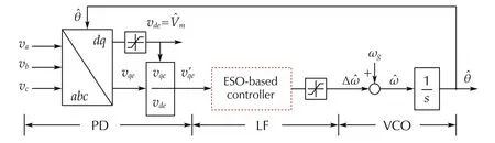
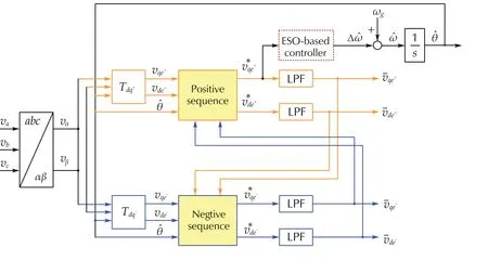
Fig. 2 Schematic diagram of ESO-based DPLL, with low-pass filter (LPF), vα , vβ the voltages in a αβ rotating reference frame, Tdq+ and Tdq- are the positive and negative sequences transforming matrices, respectively, superscript +∕- represent the positive and negative sequences components, respectively, and the upper index ‘ - ’indicates variables after filters

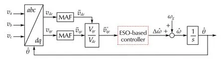
Fig. 3 Schematic diagram of ESO-based MAF-PLL, where the upper index ‘ - ’ indicates variables after filters

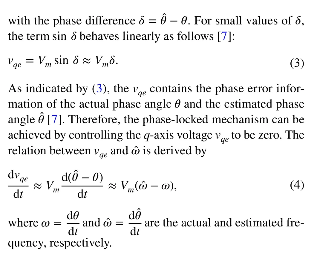
2.1 SRF‑PLL modelling

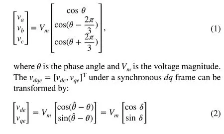
The modelling of SRF-PLL is briefly reviewed (see Fig. 1).The grid voltages are generally represented by

2.2 Extended state observer

A key procedure is to reformulate a practical control issue to the canonical model of cascade integrators with total disturbances [29]. Based on expression (4) and Fig. 4, the manipulation is conducted as follows:

A proper disturbance definition is critical to enable a highefficiency ESO [29]. Since, in the PLL, thevdeis the realtime estimation ofVm, the control gainb=Vm∕vdeapproximates 1. Therefore, the estimation of control gain is set tob0=1 . Besides, the nominal grid frequencyωgis feed-forwarded in the control input. Such operation helps improving the ESO estimation’s efficiency [29]. Finally, the total disturbancedis formulated by

2.3 Control law formulation

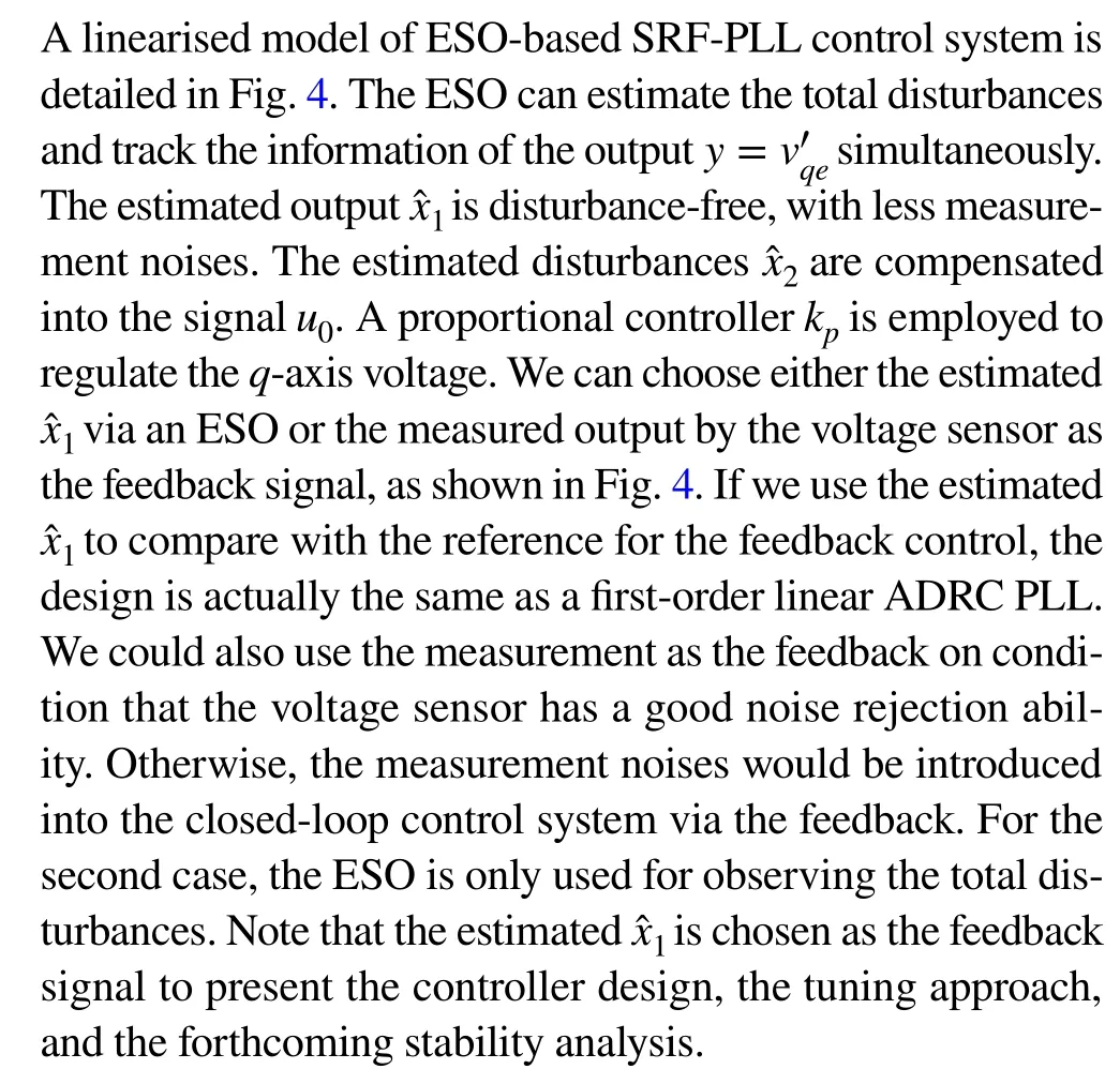
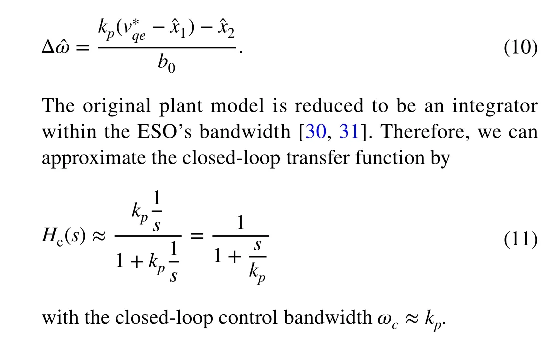
Based on Fig. 4, the control law is represented by

Fig. 4 Linearised control diagram of ESO-based SRF-PLL,β1 and β2 are the positive gains of ESO, δw is the unknown input disturbances, and b0 is the estimation of control gain

3 Tuning approach

The previous research [20] has proved that, under some conditions, a first-order ESO-based controller can stabilize the plant if it can be stabilized by a PI controller. Therefore,we can configure an ESO-based controller based on a welltuned PI controller. More importantly, such design enables a relatively fair comparison between the PI and the ESO-based controller.

3.1 Formulation of 2DOF block diagram

First, the transfer functions can be obtained from (5)-(10)as follows:

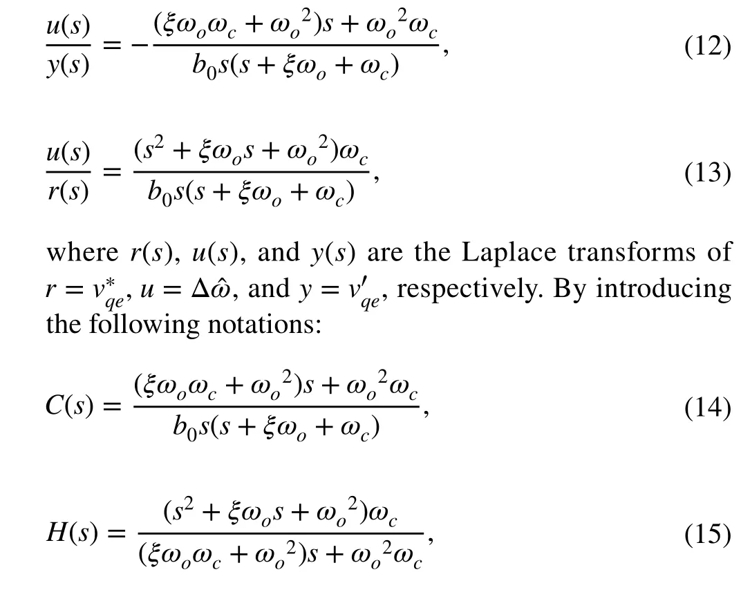
the ESO-based controller is formulated to a 2DOF closedloop system as shown in Fig. 5a. Now, we have a similar structure as a classical PI control system Fig. 5b except the prefilter. The authors of [32] indicate that the prefilter does not affect the feedback properties.

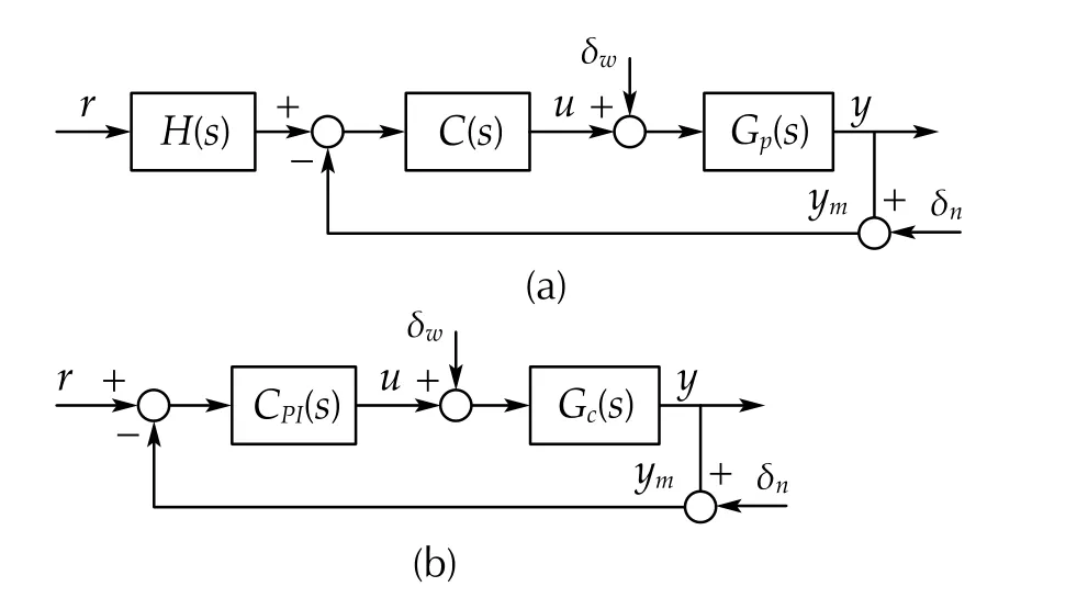
Fig. 5 a ESO-based control 2DOF diagram. b Classical PI closedloop control diagram. δw : the unknown input disturbances. δn : measurement noises

3.2 Updating ESO‑based controller with PI controller

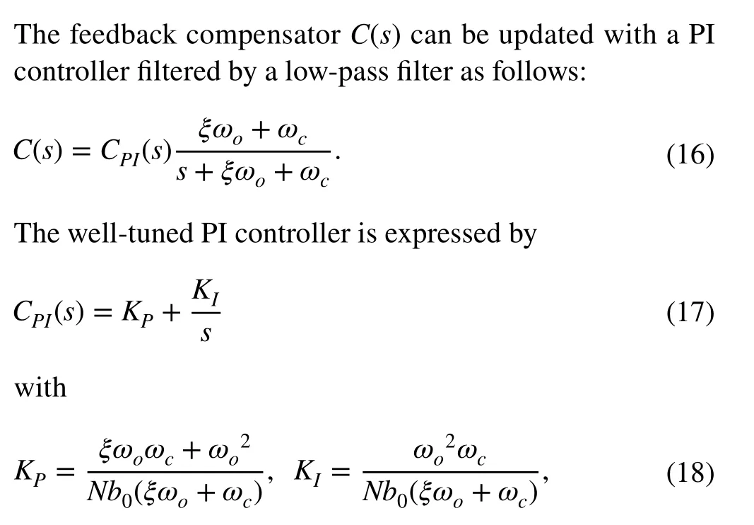
where the gain correction factorNis introduced to ensure that the ESO-based control has the similar behaviour with PI control in low frequency. By solving Eq. (18), we have

Note that the denominator (KPωo-2KI) in Eq. (19) must be positive to satisfy the stability condition, leading to the following expression:

Once the parametersξandωoare determined, the gain correction factorNcan be obtained with Eq. (18). As shown in Fig. 6, the transfer functions (14) and (16) present the same bode behaviours by introducing the gain correction factor. The gain correction factorNis introduced to ensure that the ESO-based control has the similar behaviour with PI control in low frequency. Otherwise, there would exist a constant gain difference between them. The parameters tuning guidelines will be detailed as follows.

Fig. 6 Bode diagram of C(s), CPI(s) , and

3.3 Tuning guidelines

Now, we can generate the ESO-based controller with the PI controller. Based on the above discussions, the tuning guidelines are summarized as follow:

· First, we choose the well-tuned PI parameters that have been validated in previous works.

· Regarding the parameterb0, since, in the PLL, thevdeis the real-time estimation ofVm, the control gainb=Vm∕vdeapproximates 1. It is reasonable to set the estimation of control gain tob0=1.

· The coefficientξ=2 is commonly chosen for the Hurwitz stable consideration [18]. Starting fromωo ＞ξKI∕KP, we increaseωofor Eqs. (16)-(19) until reaching noise limitations [26].

· Then, the parametersNandωcare the solutions of (18)-(19), respectively.

· Note that, for a PLL with in-loop filter, the coefficientξhas to be corrected to ensure the control stability.

· Finally, it is mandatory to validate the applied parameters of ESO-based controller in the physical tests.

The parameters of the chosen PI controllers for PLLs are given in Table 1. The parametersKPandKIfor SRF-PLL are selected based on the design method described in [7]. Besides,the well-designed parameters for the DPLL and the MAF-PLL provided in [27, 28] are considered, as well.

Table 1 Well-tuned PI parameters for different types of PLLs

4 Frequency domain analysis

The stability index is a crucial factor for evaluating the quality of a controller [10, 20, 33]. An ESO-based PLL is described in [8]; however, no detailed stabilities analyses are provided. The stability properties are, therefore, quantitatively analysed in this work. Besides, the high-frequency noise rejection ability and the closed-loop performance are analysed, as well. The noise suppression effect of ESO itself is also presented. Note that the tuning guidelines discussed in Sect. 3 will be followed in the forthcoming analysis.

4.1 Stabilities analysis

The stability of the prefilterH(s) (15) is guaranteed, as all coefficients of its denominator are positive [33]. Indeed, the prefilter does not affect the feedback properties [32]. Therefore, the closed-loop stability can be determined by the forward gain transfer function, which is given by

where the plant model isGp(s)=b∕s, andb=Vm∕vde. The stability will be analysed with respect to the observer bandwidthωo, the robustness for plant model uncertainness, and the effects of extra filters.

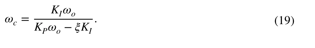
Fig. 7 Bode plots of L(s) for ωo ∈{3ωn,5ωn,7ωn}

The bode diagram ofL(s)=C(s)Gp(s) is shown in Fig. 7,withωo∈{3ωn,5ωn,7ωn} rad/s. The remaining parameters are selected by following the tuning guidelines summarized in Sect. 3. Figure 7 shows that, in low-frequency range, the ESO-based control behaves closely to the bode feature of the PI controller. Compared to the PI controller, however, its stability margin decreases due to the effect of low-pass filter.The phase margin (PM) within a range of 30◦～60◦is commonly recommended regarding the control stability [28].Therefore, the phase margin remains acceptable ( PM＞50◦).It can also be observed that the PM increases with largerωo,which can therefore enhance the control stabilities. However,theωocannot be too large, because it is limited by sensor noises and practical considerations. The parameterωomust be validated in practical conditions.

The stability of the control system can be affected by the plant model discrepancies. The main uncertain parameter for the SRF-PLL is the plant gainbas indicated by Eq. (22).The control robustness are therefore assessed under different values ofb:

The control gainb=Vm∕vdeapproximates 1, and its estimation is set tob0=1 . The bode plots of the loop transfer functionLb(s) forb∈{0.5,1.0,2.0,N,3.0} are provided in Fig. 8. The phase margin decreases when theNb0is far from the real value ofb. Though the phase margins are always acceptable.

Now, the stabilities of ESO-based PLLs with extra fillers are discussed. Regarding the DPLL, the prefilter has no direct effect on the control stability [27, 32]. However, the stability of the ESO-based MAF-PLL could be affected,because a Moving Average Filter (MAF) is placed inside the control loop (see Fig. 3). The parameters have to be corrected; otherwise, the oscillation problems would occur in the practical tests. The loop gain transfer function is modified as follows:

Fig. 8 Bode plots of Lb(s) for b ∈{0.5,1.0,2.0,N,3.0}

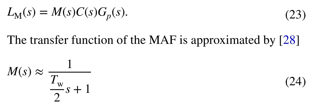
with the parameterTw=0.01 s [28].

The bode plots ofLM(s) for differentωoandξare, respectively, shown in Figs. 9 and 10. We use the following settings:ωo∈{3ωn,5ωn,7ωn} rad/s,ξ=2 for Fig. 9 andωo=5ωnrad/s,ξ∈{2,3,4} for Fig. 10. It can be seen that the PM and the gain margin (GM) decrease much due to the effect of the MAF. The PM and GM increase with a largerωo. However, theωois limited by sensor noises. The PM and GM can be enhanced using largerξ. While too largeξenables slow dynamics response [18]. Finally, the coefficientξ=4 ,ωo=5ωnis chosen for its application into the MAF-PLL.

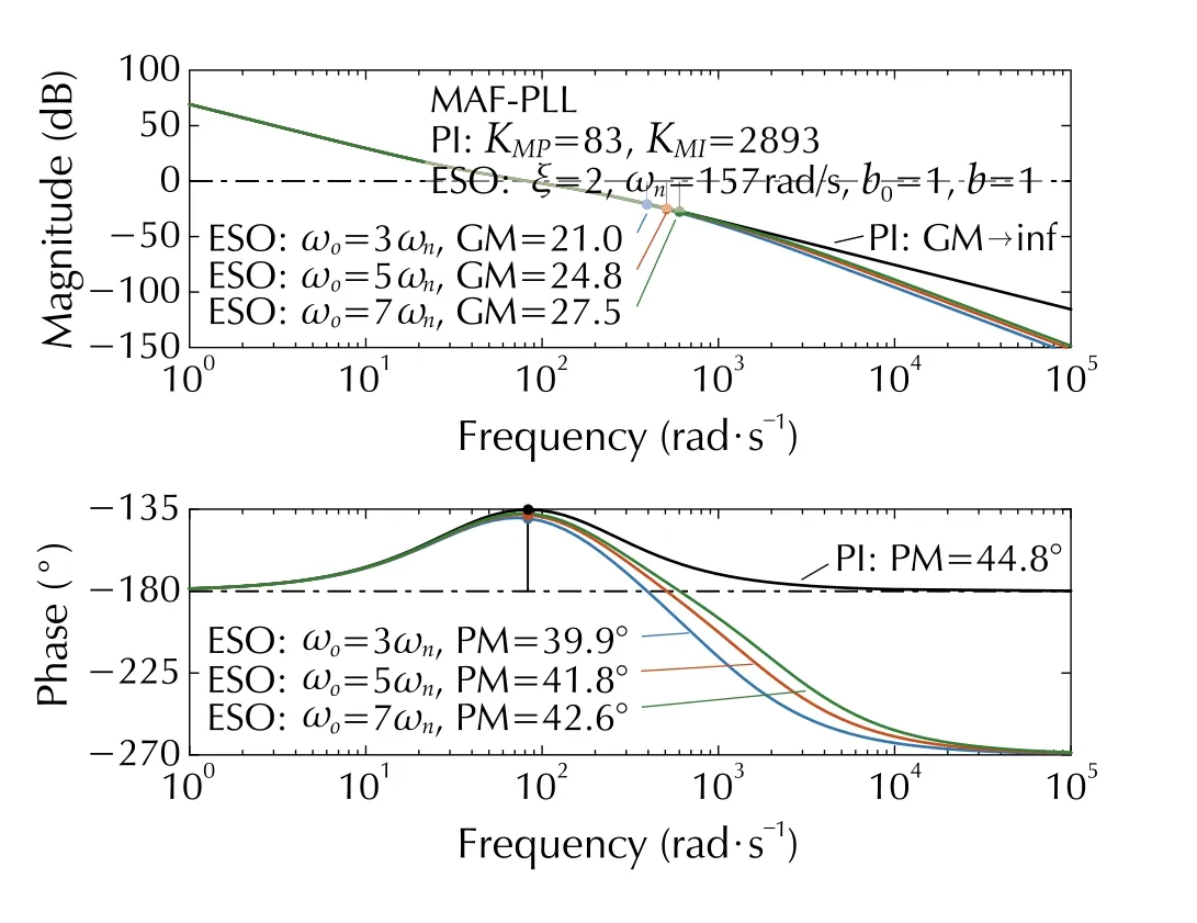
Fig. 9 Bode plots of LM(s) for ωo ∈{3ωn,5ωn,7ωn}

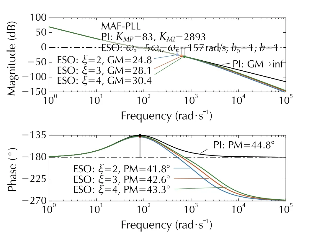
Fig. 10 Bode plots of LM(s) for coefficient ξ ∈{2,3,4}

4.2 Noises rejection analysis

As illustrated in Fig. 5, the measurement noises rejection ability is determined by the transfer function as follows:

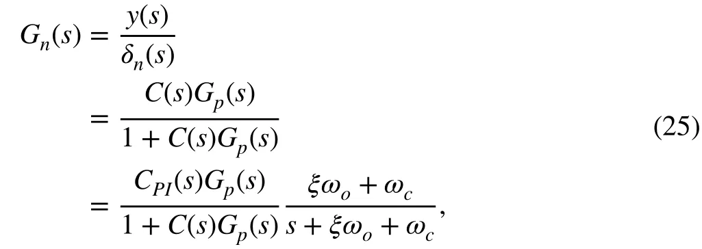
wherey(s) andδn(s) are the Laplace transforms of the outputyand the measurement noisesδn, respectively.

Figure 11 shows the bode diagram ofGn(s) . The comparative results indicate that ESO-based controller behaves better to attenuate the measurements noise compared to the PI controller. As indicted in (16), that is the low-pass filter which enhances its ability to reduce high-frequency noises. Besides,the noise rejection ability decreases when the parameterωoincreases.

Now, we discuss the noise attenuation effect of ESO itself.Based on Eqs. (7)-(10), the transfer function of the estimated state variable1is obtained as follows:

Then, theresulting from the measurement noiseδnand the input disturbanceδwcan be given by

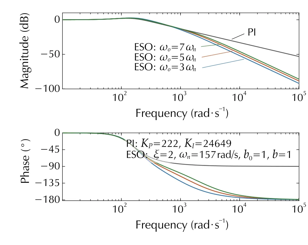
Fig. 11 Bode plots of Gn(s) for ωo ∈{3ωn,5ωn,7ωn}

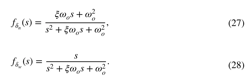
The bode plots offδn(s) andfδw(s) are shown in Figs. 12 and 13, respectively, withωo∈{3ωn,5ωn,7ωn} rad/s. It can be observed from Fig. 12 that the ESO performs as a low-pass filter, which can reject the high-frequency signals. Besides,the largerωocan increase the high-frequency gain. Namely,the ESO would be more sensitive to the high-frequency measurement noise when we increase theωo. It can be seen from Fig. 13 that the phase lag ofis decreased with largerωo; however, there is no influence on the high-frequency gain; the ESO can more efficiently attenuate the input disturbance in the low-frequency region. Consequently, there exists a trade-off between the input disturbance rejection and the measurement noise sensitivity [34].

Fig. 12 Bode diagrams of the transfer function fδn(s) for ωo ∈{3ωn,5ωn,7ωn}

Fig. 13 Bode diagrams of the transfer function fδw(s) for ωo ∈{3ωn,5ωn,7ωn}

Based on (9), the transfer function of disturbances estimation error becomes

The bode plots offe2(s) are shown in Fig. 14, withωo∈{3ωn,5ωn,7ωn} rad/s. The ESO can estimate the unknown disturbance very well only when the disturbances are composed of low-frequency components [10]. The disturbance estimation errors can be reduced by increasing theωo; however, theωois limited by the noises sensitivity.

4.3 Closed‑loop performance analysis

Based on the formulated 2DOF diagram (see Fig. 5), the closed-loop transfer function of the ESO-based PLL is represented as follows:

The bode plots ofGcl(s) are shown in Fig. 15. The closedloop performances of PI and ESO-based control system behave closely at the low-frequency range. It can also be noticed that there is a peak greater than 0 dB for the PI control system, which indeed corresponds a time-domain overshoot of the step response [20]. However, for the ESO-based control, the overshoot is attenuated due to the prefilter H(s).

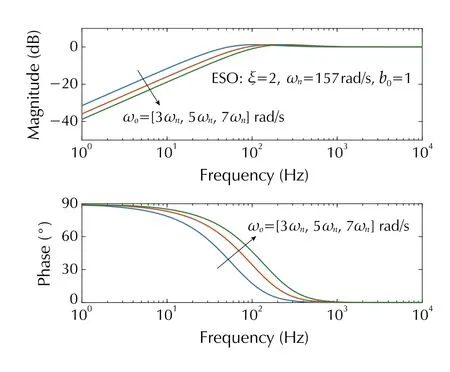
Fig. 14 Bode diagram of the transfer function fe2(s) for ωo ∈{3ωn,5ωn,7ωn}

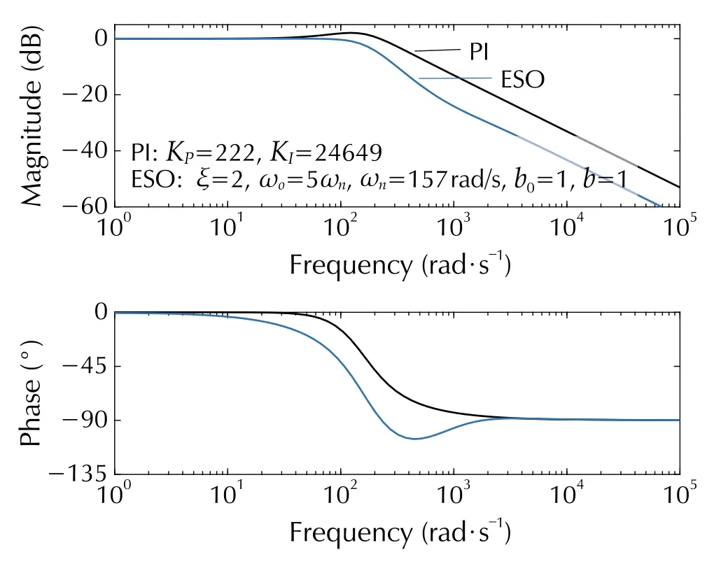
Fig. 15 Bode plot of closed-loop transfer function Gcl(s)

5 Simulation studies and results

Simulation studies are conducted with the Matlab/Simulink.We use the solver Ode3 (Bogacki-Shampine) with a fixed step size 0.1 ms [8]. The balanced three-phase voltages are set toVm=179 V,f=50 Hz. A white noise is manually added to simulate the voltage measurement noises. The ESO-based SRF-PLL/DPLL/MAF-PLL are, respectively,simulated by considering different disturbed regimes. The parameters of ESO-based PLLs are selected by following the tuning guidelines in Sect. 3; meanwhile, the control stability is taken into account, as well. The control parameters of ESO-based SRF-PLL and DPLL are set toωo=5ωnrad/s,ωn=157 rad/s,ξ=2 , andb0=1 . Regarding the MAF-PLL,the coefficientξ=4 is applied to ensure the control stability,and the remaining parameters are set to the same as those of the SRF-PLL.

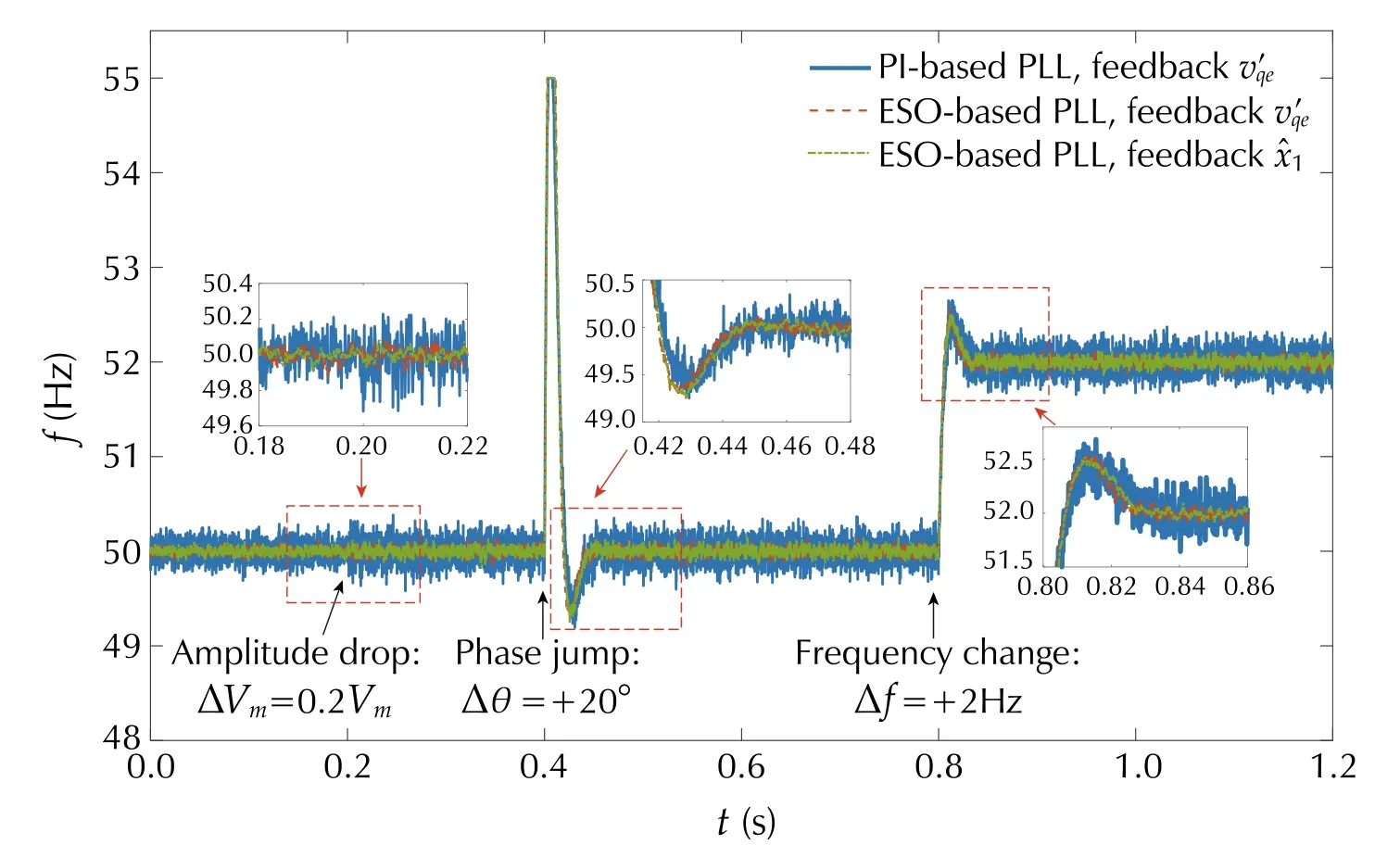
Fig. 16 Estimated frequencies of ESO-based SRF-PLL

Fig. 17 Phase tracking errors of ESO-based SRF-PLL

The unbalanced case is tested to assess the effects of the extra filters on the ESO-based LF. Figures 18 and 19 show the performances of ESO-based DPLL and MAFPLL. The voltage unbalances happen att=0.2 s, and the unbalanced voltages are set toVam=Vm,Vbm=0.8Vm,Vcm=0.8Vm. A phase jump of +20◦is induced att=0.4 s.The grid frequency varies from 50 Hz to 52 Hz att=0.8 s.The simulation results for PI controllers are also provided for the comparisons. Some conclusions are suggested by the results, as shown in Figs. 18 and 19. First, the ESO-based DPLL and MAF-PLL present almost the same dynamic responses as the corresponding PI control for tracking the information of the frequency and the phase. Then, as the MAF itself could help attenuate the high-frequency noises,consequently, the advantage of ESO-based LF when applied to the MAF-PLL is not very significant. Moreover, the DPLL performs faster response dynamics compared to the MAF-PLL. Therefore, in the following part, only the ESObased DPLL is implemented into the closed-loop control of the GcC.

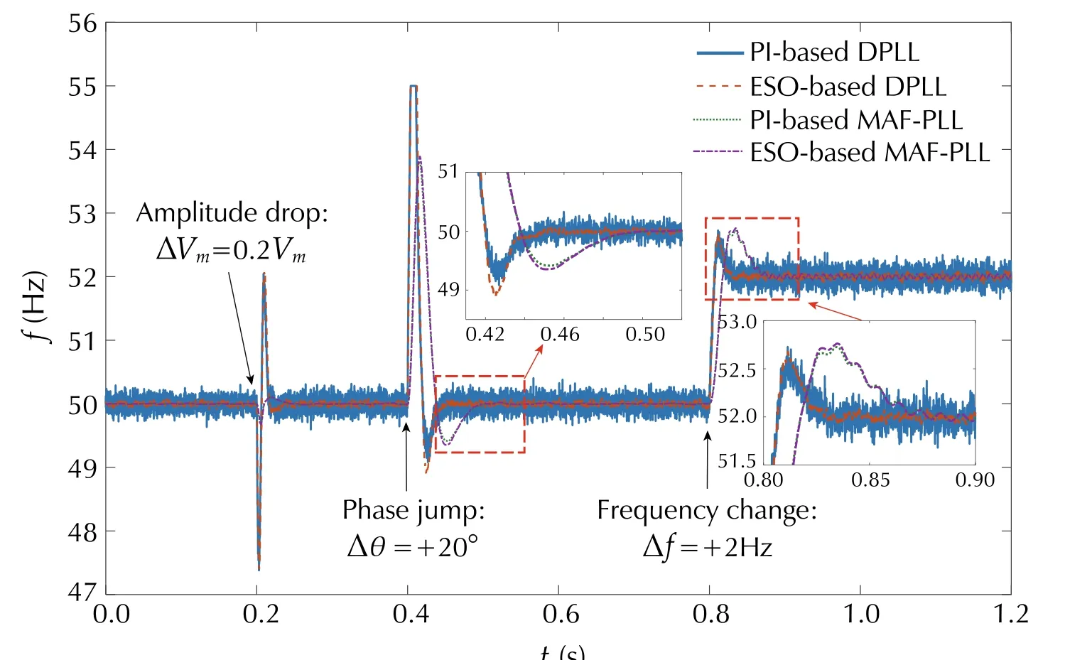
Fig. 18 Estimated frequencies of ESO-based DPLL and MAF-PLL

Fig. 19 Phase tracking errors of ESO-based DPLL and MAFPLL

6 Experimental tests and results

The closed-loop control performances of GcC equipped with ESO-based PLL are experimentally validated in this section.Experiments are conducted in a real-time hybrid PHIL test benchmark, as schematically illustrated in Fig. 20, which consists of the three-phase grid-connected converter, the disturbed grid emulator [35], and the dSPACE hardware (DS1005) [36].The three-phase GcC is a back-to-back Pulse Width Modulation (PWM) voltage source converter. The control signal is converted to the PWM command for the converters in real time[36]. The disturbed grid is emulated by the RT-LAB real-time digital simulator [8]. Key parameters of the testing benchmark are listed in Table 2.

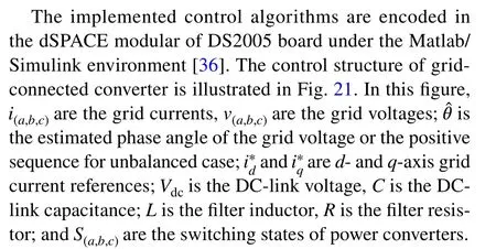
The control of GcCs mainly has three functions: the grid synchronization [8], the DC-link voltage control [37],and the grid current control [38]. First, the outer voltage loop maintains the constant DC-link voltage, where a PIcontroller is used in this work. Then, the proposed ESObased PLL is used to obtain the grid voltage phase to synchronize the injected current with the grid voltage. Furthermore, the injected current control is achieved through three Proportional Resonant (PR) controllers upon theabcthree-phase frame. More design details with respect to the control designs of GcCs can be found in the previous literatures [37-39]. Regarding the unbalanced conditions, various control strategies have been proposed before [40, 41].In our tests, we use the positive sequence control strategy proposed in [40]. The PLL is used to detect the phase angle that follows the positive sequence of the grid voltage. For the ESO-based PLLs, we keep the same control parameters as configured in the simulation studies. The well-tuned parameters of the PI controller for the DC-link voltage and the PR controllers for grid-injected currents are provided in Table 3, and the detailed definitions of these parameters can be found in [9]. Since there is no difference between the synchronization phase angle during the unbalances and that during normal grid conditions, the same control parameters values are thus used for both balanced and unbalanced cases.

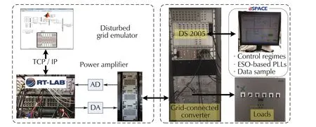
Fig. 20 PHIL experimental benchmark

Table 2 Parameters of the experimental benchmark

Figure 22 presents the closed-loop control performances of GcC equipped with ESO-based PLL/DPLL. Figure 22a shows the control performances under balanced grid. Testing results for unbalanced grid are provided in Fig. 22b. To highlight, we suppose that the unbalance is not affecting the phases but the magnitudes only. Then, the positive sequence is synchronized with the phase “a” of the original threephase voltages. Therefore, the estimated phase of the positive sequence follows the original phase angle.

The test conditions are set as follows: a phase jump of+20◦is manually added in Fig. 22a1 and b1, a frequency step of 2 Hz happens in Fig. 22a2 and b2, and an magnitude drop of 0.2Vmis considered in Fig. 22a3 and b3. First, theESO-based SRF-PLL/DPLL can correctly follow the phase,the frequency, and the voltage amplitude information. Then,the results indicate that the injected grid currentiasynchronizes with the grid voltageva. Furthermore, the GcC’s controls equipped with the ESO-based SRF-PLL/DPLL enable efficient performance regarding the control dynamics and the robustness in the presence of various disturbances.

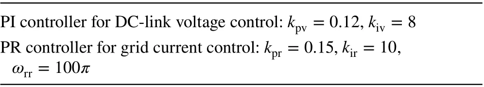
Table 3 Control parameters of grid-connected converter

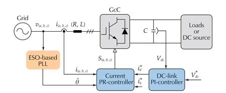
Fig. 22 Grid-connected control performances with ESO-based PLL/DPLL under balanced and unbalanced grid conditions, the grid current of phase a ia (2A/div), the grid voltage of phase a va (100 V/div), for a1 and b1, a phase jump of Δθ =+20π∕180 rad, the actual voltage phase θ(2rad/div), the estimated voltage phase (2rad/div); for a2 and b2, a frequency step of Δf =+2 Hz, the actual grid frequency f (1Hz/div), the estimated grid frequency (1Hz/div); for a3 and b3, a voltage magnitude variation of ΔVm =0.2Vm , the d-axis voltage vde (20 V/div), and the q-axis voltage vqe (20 V/div). (a1)-(a3) Balanced grid voltages. (b1)-(b3) Unbalanced grid voltages

7 Conclusions

This work is an extension for our previous work [8]. A linear ESO-based controller is designed as the LF for the SRFPLL. A tuning approach based on the well-tuned parameters of PI controller is provided, which results in a fair comparison with PI-type PLLs. Some conclusions can be drawn from the frequency domain analysis and the simulation results:the performances of the generated ESO-based controller are close to those of PI control at low frequency, while achieving a better ability of attenuating measurement noises. The phase margin decreases slightly, but remains acceptable. For the MAF-PLL with the in-loop filter, the equipped MAF itself could help attenuating the effects of high-frequency noises. Consequently, the advantage of ESO-based LF for its application to the MAF-PLL is not very significant. The PHIL experimental results suggest that the ESO-based PLLs can correctly obtain the phase, the frequency, and the voltage amplitude information. The obtained results show the effectiveness of ESO-based PLLs when applied to the GcC in the presence of various disturbances.

It is worth mentioning that this work has discussed a tuning approach based on the well-designed PI control. However, for the implementations of ESO-based control, it is not mandatory to tune them based on a PI controller. The linear ESO-based controller can be tuned simply by following the parameters selection guidelines provided in the previous works [8, 18, 21].

AcknowledgementsThis paper was supported by G2elab, Grenoble INP, University Grenoble Alpes, France and School of Engineering,HES-SO, Valais, Switzerland.

FundingOpen Access funding provided by Haute Ecole Specialisée de Suisse occidentale (HES-SO).

Open AccessThis article is licensed under a Creative Commons Attribution 4.0 International License, which permits use, sharing, adaptation, distribution and reproduction in any medium or format, as long as you give appropriate credit to the original author(s) and the source,provide a link to the Creative Commons licence, and indicate if changes were made. The images or other third party material in this article are included in the article’s Creative Commons licence, unless indicated otherwise in a credit line to the material. If material is not included in the article’s Creative Commons licence and your intended use is not permitted by statutory regulation or exceeds the permitted use, you will need to obtain permission directly from the copyright holder. To view a copy of this licence, visit http:// creat iveco mmons. org/ licen ses/ by/4. 0/.