Data‑driven disturbance observer‑based control: an active disturbance rejection approach

Harvey Rojas‑Cubides · John Cortés‑Romero · Jaime Arcos‑Legarda

Abstract

Keywords Active disturbance rejection control · Data-driven disturbance observer · Disturbance observer-based control ·Signal prediction

1 Introduction

External disturbances, measurement noise, parameter uncertainty and unmodeled dynamics are the most common issues in the design of robust control strategies. For decades, each of these aspects has been handled independently. However,starting in the 90s, based on the work of J. Han, a unified approach to deal with all these adverse effects, which lumps internal and external disturbances, including the unmodeled dynamics, into a concept called total disturbance was developed [1, 2]. This concept joined to the mechanisms for its estimation and compensation is the core of the active disturbance rejection control (ADRC) approach [3, 4].Besides, total disturbance idea is closely related to lumped disturbance or equivalent input disturbance in the context of disturbance/uncertainty estimation and attenuation techniques [5].

Under this approach, external disturbances, uncertainties and unmodeled dynamics are considered as a lumped disturbance, which is attenuated with a disturbance rejectionbased control. This technique is widely used to improve the robustness of feedback controllers against external disturbances and model uncertainties. The methods to perform disturbance rejection control can be grouped, according to their design approach, into three main categories: (1) timedomain, (2) frequency domain, and (3) data-driven.

The first method, the time domain-based design, uses the state-space representation of the system model to assign additional states that represent the internal dynamics of the disturbance signal. In this way, a state observer is designed to estimate all the states of the model, including the states that represent the disturbance signal and its internal model.There are several observer strategies that are used this approach: the extended state observer (ESO) [6, 7], active disturbance rejection control (ADRC) [8], generalized extended state observer (GESO), also known as generalized proportional integral (GPI) observer [9, 10], unknown input observers (UIO) [11], and high-gain observer (HGO) [12].

The second method uses the frequency domain analysis. The main structure of this method is the disturbance observer (DOB), which usually uses a plant inverse and a Q-filter design that ensures a causal realization of the observer [13]. The main drawbacks of this method is the use of the plant inverse, which might be an unstable inverse if the system is non-minimum phase. This problem has been addressed for several researchers that have proposed the use of stable inverse [14]. To mitigate the design efforts of the plant inverse and the Q-filter necessary into the conventional DOB’s structure, Zheng et al. [15] proposed a generalized design method that minimizes the norm of the dynamics from disturbance to its estimation error. The digital implementation of the DOB entails the Q-filter implementation, which is generally designed as a digital versions of basic analog filters [16, 17], zero-phase low-pass FIR filter[18, 19], discrete binomial filters [20] and infinite impulse response filters [21-23], among others.

The third method uses data-driven techniques. These methods do not necessarily consider the explicit system models or the disturbance internal model. Instead, it uses the input-output data to predict the trend of the disturbance signal [24]. This paper explores the third method with a novel data-driven disturbance observer. Despite of the huge number of scientific contributions on disturbance observers, there are very few reports exploring the opportunities that the data analysis and signal processing could produce into the area of disturbance estimation. This issue has been approached using the disturbance history data to solve a least square regression problem that fits the disturbance signal history to a polynomial basis function, which, in the sense of Taylor’s series, is the most effective and simplest methods for curve fitting [25-27]. Moreover, the time series expansion and the Moore-Penrose pseudoinverse has been used to estimate higher order disturbances in nonlinear systems [28].Besides the curve fitting, data information has been used in learning strategies to enhance the DOB’s performance under quasi-periodic disturbances [15]. In this way, techniques, such as iterative learning control [29, 30] have been developed to attenuate the effect of periodic disturbances;however, the learning process hardly guarantees stability in the transient responses.

This paper proposes a control based on a data-driven disturbance observer (3DOB), which guarantees stability in the transient response through an inner control loop. Additionally, the approach used by the 3DOB to estimates the disturbance does not require explicit design of the plant inverse or a Q-filter. Thus, this approach eliminates the structural constraints of the conventional DOB. The remaining of this paper is organized as follows: Sect. 2 describes the general outline of the proposed approach. Section 3 presents the data-driven disturbance observer structure. Section 4 shows the proposed predictor scheme that is the essential part of the data-driven disturbance estimation and rejection. Section 5 presents design criteria and stability-performance analysis.Section 6 shows the experimental validation of the control strategy on a switched DC-DC synchronous buck converter.Finally, Sect. 7 summarizes the accomplishments of this work and draws recommendations for future developments.

2 Proposed approach

A general outline of the proposed approach is presented in Fig. 1. Consider a minimum phase plant described by the following discrete time model that relates the measurable outputy(k) and the control inputu(k):

wherenis the system order, andNG(z) andDG(z) are polynomials in thezdomain. In addition, systemG(z) is perturbed by an equivalent input (total) disturbanceξ(k) which includes all endogenous and exogenous adverse effects.Therefore, the goal is to design a control system that allows robust tracking of the referencey*(k).

The proposal is defined under the general disturbance estimation and attenuation approach, and particularly in the context of the active disturbance rejection control framework. Likewise, the control strategy is completely presented in discrete time, avoiding the use of discretization methods for its digital implementation, e.g., a bilinear transformations.

In general terms, the proposed strategy is divided into two stages: inner or stabilization loop and outer or filter-prediction loop. The purpose of the inner loop is to stabilize the system dynamics while adjusting its internal model. This allows, on the one hand, to design a complementary disturbance rejection scheme and, on the other, to adjust a robust tracking according to the internal model considered. A key point in the inner loop is the definition of a disturbance signal equivalent to the output(ξ1) that can be synthesized thorough knowledge of the available output and an auxiliary control input (u1). This equivalent disturbance signal will be processed as part of the synthesis of the outer loop controller.

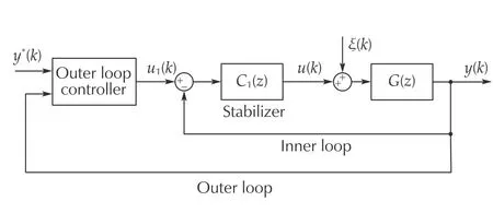
Fig. 1 General control scheme for the proposed approach

The outer loop is inspired by the guidelines of a control structure based on a disturbance observer, where for this case,the inverse of the equivalent system resulting from the inner loop is required. As usual, this inverse corresponds to an improper transfer function causing implementation problems due to dependence on future values. Precisely, those related predictions associated with the equivalent disturbance can be estimated online based on a polynomial approximation of the trend associated with the data-signal history in the Taylor sense.

2.1 Stabilization using the inner loop controller

Consider the plantG(z) described in (1) and a unified equivalent disturbance to the control inputξ(t) such that The degree and structure of the controllerC1(z) is such that it allows, on the one hand, the arbitrary location of the roots of the polynomialD1(z)=DC1(z)DG(z)+NY(z)NG(z) and, on the other hand, the rejection of structured disturbance signals whose internal models have been considered in theC1(z)design. As initial requirement, the numerator resulting from the controller,NC1(z) , must have its roots within the unit circle of the complex plane. In the event thatNC1(z) exhibits unstable roots, an additional procedure must be performed.This restriction can be easily manipulated from the algebraic point of view through a two-degree of freedom control structure [31]. For this purpose, the following subsection proposes an adaptation of the two-parameter compensator.

At this point, it is important to highlight that the system obtained from the internal loop is stable and it also has the ability to track or reject the signals that are included in the internal model considered inC1(z).

2.2 Two‑parameter compensator issue

As previously indicated, a requirement in the inner loop is that theNC1(z) polynomial has stable roots for a stable model-inverse when formulating the control law. This problem can be solved by including the classic two-parameter compensator presented in Fig. 2.

The proposed approach follows, in the first stage of the design, the model matching methodology to impose a stable numerator in the resulting control system.

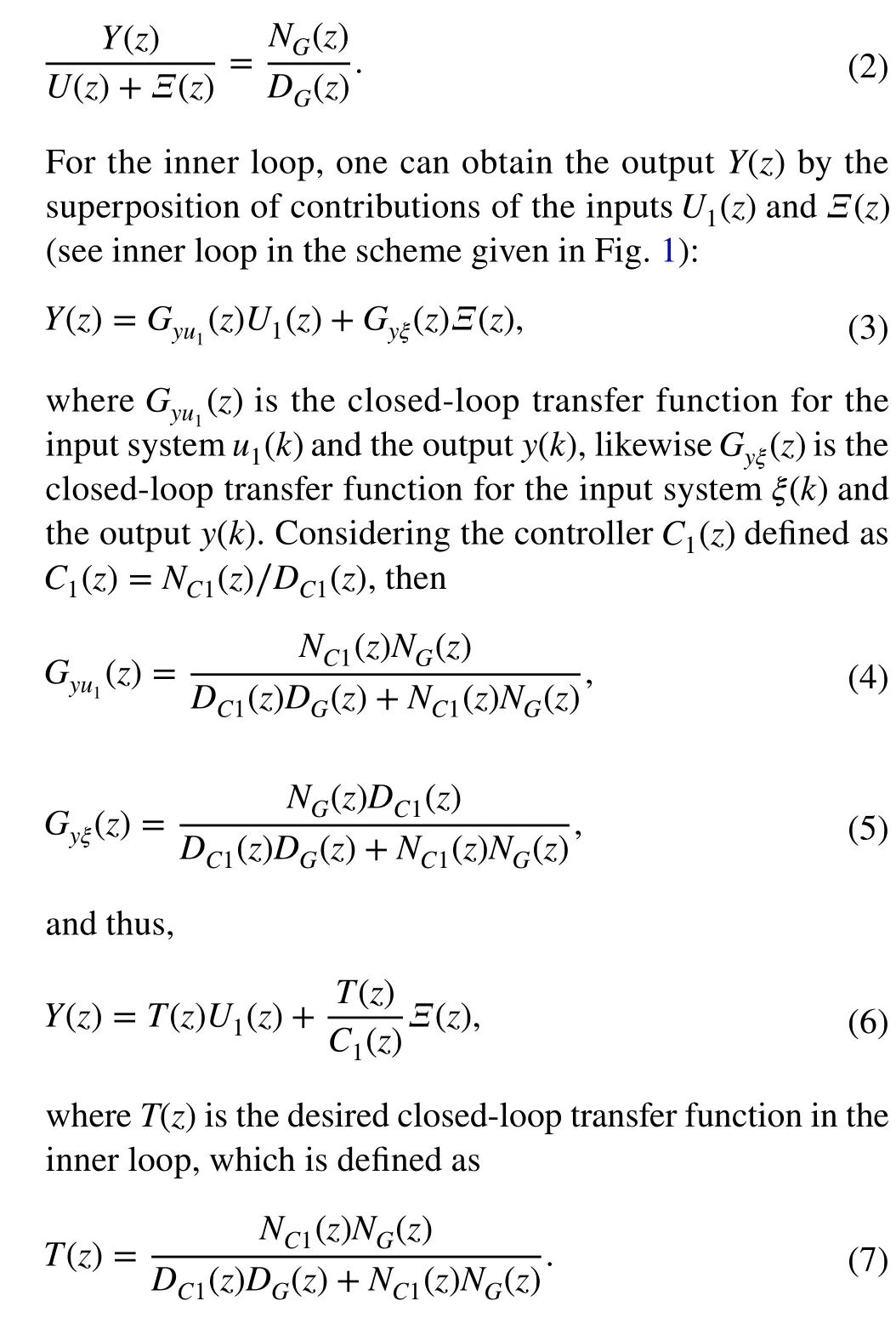
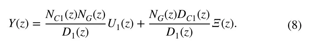
Under the current methodology, a two input-one output dynamics is considered as in Eq. (6):

Hence, the intent of using the two-parameter compensator is to match the transfer function of the control system to a desirable numerator and denominator model, both with stable roots by construction. The first is to implement a stable inversion and the second is to achieve arbitrary pole placement.

A supplementary polynomialNU1(z) is imposed through the following control law:

Fig. 2 Two-parameter controller structure

Remark 1In the following,K1(z) can be used instead ofC1(z) when a two-parameter controller procedure was not necessary, and the design is based on the inner loop diagram presented in Fig. 1.

Once a suitable stabilization has been carried out by means of the internal loop, an outer loop based on a datadriven disturbance observer is proposed.

3 Data‑driven disturbance observer

To find a simplified equivalent disturbance signal in the outer loop, let us defineΞ1(z)=Ξ(z)∕K1(z) as a filtered version of the equivalent disturbanceΞ(z) . This is,

Then a useful characteristic definition of the new filtered disturbance, justifying the application of the stabilization loop, can be obtained online by a simpley(k),u1(k) processing, i.e.,

Hence, an ideal and non-implementable control law forU1(z)is given by

whereT-1(z) is an improper transfer function that demands future values ofY(z) causing implementation problems. This general math definition, bears similarity with the idea used in the classical disturbance observer design (in an inner loop); however, in this work, a different way to deal with this problem is presented as described below.

Definingras the relative degree ofT(z) and to obtain an implementable version of (18), a delayed version of the disturbanceΞ1(z) is proposed as

Nevertheless, up to this point only ar-delayed version (not the current one) of the disturbanceξ1(k-r) is available.For this reason, a data-driven predictorP(z) that estimates the current version of the disturbance(k) is included as follows:

The proposed control scheme is shown in Fig. 3. This scheme is composed of an inner loop together with a data-driven disturbance observer in the outer loop. The inner loop includes a Two-parameter compensatorK(z)=[K1(z) -K2(z)]designed to obtain a desiredT(z), based on the nominal/known model of the plantG(z) and assuming a perfect disturbance rejection. On the other hand, the disturbance observer in the outer loop uses the reference transfer functionT(z) and itsr-delayed inversez-rT-1(z) (winch is a proper transfer function) to obtain ar-delayed disturbanceξ1(k-r) . Finally, a predictor schemeP(z) is included to achieve an estimation of the current disturbance(k).

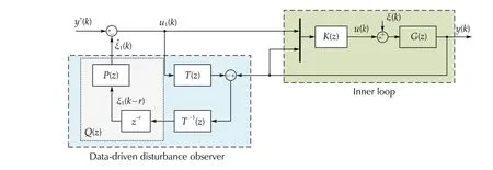
Fig. 3 Proposed control scheme

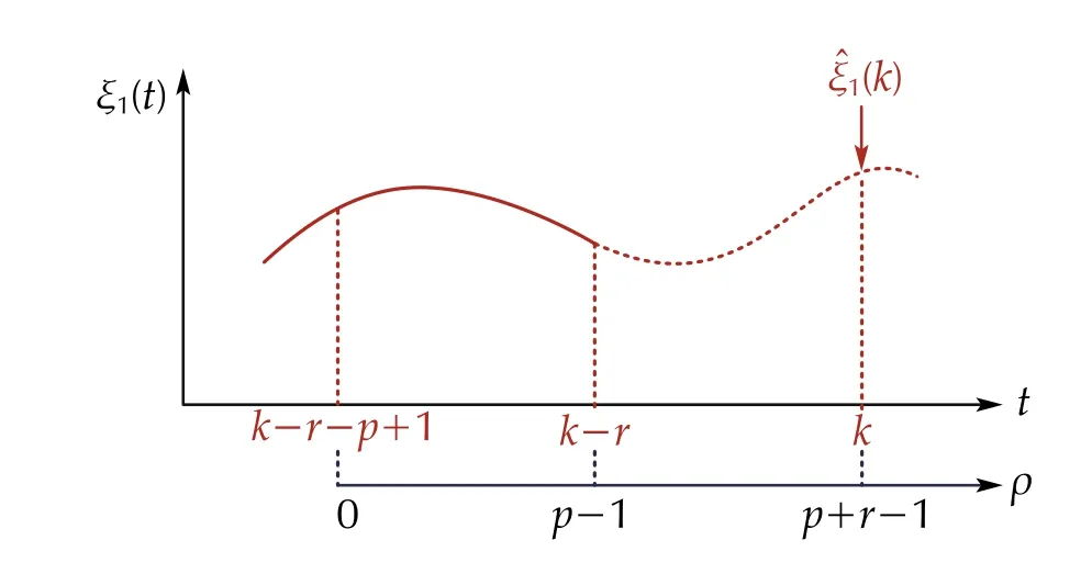
Fig. 4 Prediction process

4 Predictor scheme

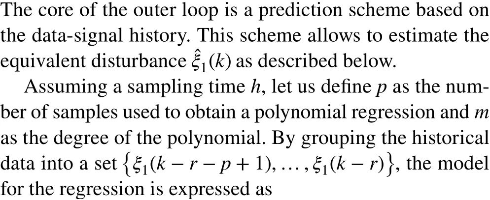
An excess in the number of samplespover the order of the polynomial regressionmis required to obtain a low-pass filter effect. The criteria for this adjustment involve the knowledge of noise level of the signals, sampling time, and bandwidth.

According to the previous analysis, it is possible to define the family of transfer functions for the predictorP(z) given by

5 Design criteria and stability‑performance analysis

To analyze the effect of the data-driven disturbance observer over the system performance and stability, the control law(22) is replaced in the output dynamics (15) as follows:

whereQ(z)=z-rP(z) . From this expression, it can be inferred thatTQn=Q(z) , andSQn=1-Q(z) represent the complementary sensitive and sensitive functions of the estimation process, respectively. Now, using the predictor transfer function (26), we have

5.1 Closed‑loop stability

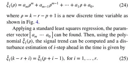
With the aim to explore the closed-loop stability analysis,equation (29) is rewritten as

which allows to draw the following observations about closed-loop stability.

On the one hand, the inner loop process design guarantees the stability of the transfer functionT(z). On the other hand,given the structure of the obtained predictor, the equivalent function 1-Q(z) places its poles at zero, which also assure its inherent stability. Therefore, (35) presents a linear dynamic system with two inputs one output, predominantly governed by two stable transfer functions.

The inner loop, called the stabilizer loop, is in charge of the stable priming structure of the overall control system.As conceived in the proposed two-stage ADRC approach,the outer loop performs an estimation and consequent rejection of the EID while preserving the stable structure imposed by the inner loop. This property remains invariant only for adequate performance of the equivalent DOB. In fact, the proposed strategy can be viewed as robust feedback linearization scheme. The validity of the resulting linearization is directly proportional to the effectiveness of the rejection of the unified disturbance. This can be expressed simply (frequency domain) since the DOB must comply with a minimum bandwidth. Once this requirement is fulfilled, the linearization of the system is achieved and one could even speak of separability.

It is worth to note that according the ADRC framework,every mismatch of the model based of the design with respect to the real behaviour of the system can be included into the unified total disturbance. Therefore, missing nonlinear dynamics or related uncertainties are also considered as part of the lumped disturbance and can be handled by the proposed method.

On the other hand, a deeper non linear robust stability analysis can be difficult issue and it is out of the scope of the present work, see, e.g., [32]. However, a simple stability analysis, based on the linearization process, like the one presented in this work could be favorable in an practical engineering context [33]. In this sense, even though in this paper has not given an exhaustive result related with the specific effect of nonlinear uncertainties, owing to mathematical complexity, the main features of the proposed approach and its efficacy has been illustrated using experimental results.

5.2 Design parameters and performance

According to the equation (32) and the block diagram presented in Fig. 3, it is possible to establish that transfer functionQ(z)=z-rP(z) fulfills a similar role as the Q-filter in the classical disturbance observer-based control (DOBC) [20],or an extended state observer in the ADRC framework [34].However, the proposed approach focuses on the design of a data-driven observer based on a predictor. Nonetheless,this work takes advantage of the similarities with DOBC,using some well-known frequency domain analysis tools.This facilitates the robustness-performance analysis and it makes the choice of the design parameters clearer.

The tuning parameters of the data-driven disturbance observer are: the polynomial orderm, the number of samplespin the predictor, and the sampling period (in some cases). Thus, for each combination in the design parameters,the predictor is represented by a different transfer function(P(z)) and the frequency response of the observer changes.This feature shows the flexibility of the proposed approach.To present the properties of this strategy, Figs. 5 and 6 show the frequency response ofQ(z) forr=1 and some combination ofmandp.

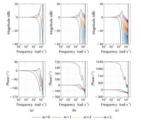
Fig. 5 Frequency response of Q(z) varying the polynomial order for 5, 10 and 20 samples p, and h=20 μs

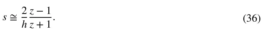
An additional feature shown in Fig. 6 is the effect of number of samples over robustness and performance.Here, a low number of samples achieve better performance in low frequency, but the bandwidth is higher causing issues with the noise. While, a larger number of samples produces a low-pass filter effect; and however, this also produces a lower performance.

5.3 Equivalence of Q(z) in the S‑domain

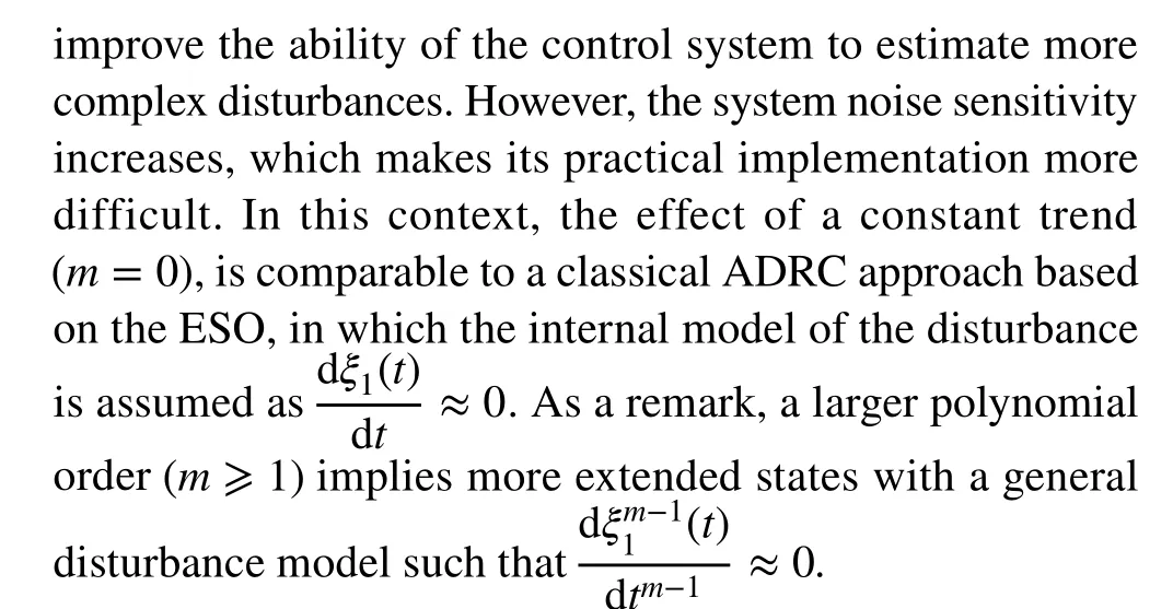
It is possible to establish an equivalent in the S-domain for the final results obtained in this work. For instance,using a bilinear transformation ofQ(z), where for a given sampling periodhwe have

As an example, Fig. 7 presents the frequency response ofQ(z) and its equivalent in the s-domainQ(s) (based on the bilinear transformation) for three combinations of design parametersmandp, forr=1 andh=20 μs.

The results show that it is conceivable that under a certain design and with an appropriate tuning, a Q-filter could be obtained with a similar performance as presented in this work, at least in the zone of low and medium frequencies.However, it is clear that this continuous-time design would not correspond to a data-driven approach, which is the core of this work.

6 Experimental validation

With the aim to validate the proposed control strategy, the case of a switched DC-DC synchronous buck converter (SBC) is considered. This kind of converter produces a regulated output voltage that is lower than its input voltage, and can providehigh currents while improving the efficiency. As shown in Fig. 8, a generic SBC is comprised mainly of an input voltage sourcevi, two power MOSFETs controlled with PWM (with their gate drivers), an LC output filter, and the load resistance.The simplified average dynamic model of a buck converter for voltage-mode control is described as

Fig. 6 Frequency response of Q(z) varying the number of samples for polynomial order m=[0,1,2] , and h=20 μs

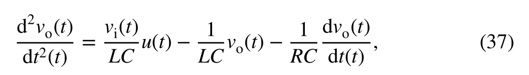
whereRis the load resistance of the converter,Lis a filter inductance,Cis an output capacitor,vi(t) is the input voltage,v0(t) is the average output capacitor voltage, and the duty cycleu(t)∈[0,1] represents the control signal.

Some elements that motivate the use of this platform to test the control proposed approach are (1) synchronous buck DC-DC converter is a hybrid system, given the switching mode of the circuit. Moreover, there are several commonly unmodeled nonlinear effects, such as magnetic characteristics of the inductor, electro-magnetic interference caused by switching and dead time, among others, which have influence in the control performance [35]. (2) The system components values can undergo changes during its lifetime,which cause a relevant uncertainty factor for output voltage regulation [36]. (3) During its normal operation, the system is affected both by matched disturbances at the control channel (input voltage changes), as well as, by mismatched disturbances caused by current load changes. This fact, is often a challenge for the control strategies under the ADRC and DOB approaches [37]. (4) The voltage-mode for buck converters is characterized both by its simplicity due it no need to sense the inductor current, and also its low openloop output impedance. However, it has some disadvantages due its poor line rejection and because control-to-output transfer function changes between operating modes; therefore, a disturbance estimation and rejection scheme could be useful [38]. (5) Taking into account its real applications,such as motor drivers, chargers for electric vehicles and DC transmission, among others, it is desirable to achieve a direct digital controller with an easier and cheaper implementation in standard electronic devices, e.g., a microcontroller [39].

Considering the above, the main challenge is to find a control law such that the output voltagev0(t) is forced to track the given referencev*o(t) , even in presence of disturbances, such as changes in the load, input voltage variations,uncertainties in electronic components and non modeled dynamics, among others.

Fig. 7 Frequency response of Q(z) and its equivalent in the s-domain varying the design parameters, for r=1 and h=20 μs

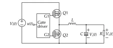
Fig. 8 Circuit diagram of DC-DC synchronous buck converter

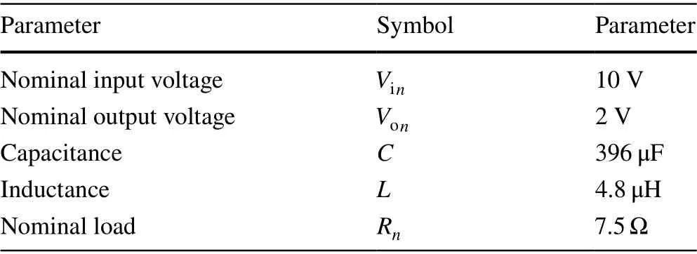
Table 1 Parameter of the DC-DC synchronous buck converter

6.1 Experimental setup

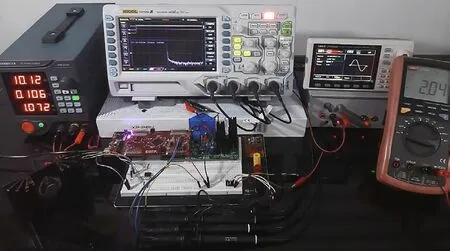
Fig. 9 Experimental setup including (1) DC-DC synchronous buck converter with active load, (2) 32-bit floating-point microcontroller,(3) Programmable DC power supply, (4)-(6) system to generate the input voltage disturbances, (7) and (8) measuring instruments

The experimental test setup configuration and the prototype are depicted in Fig. 9. In general terms, the platform includes: (1) the power stage composed by a DC-DC synchronous buck converter with active load,(2) a 32-bit floating-point microcontroller unit (MCUTMS320F28377S) to implement the control algorithms using Code Composer Studio v10.1 and Matlab v2020a,(3) a programmable desktop laboratory DC power supply(HM305) with the measurement of voltage, current and power in the input side of the converter; a system to generate the input voltage disturbances that includes: (4) an arbitrary waveform generator (UTG932E), (5) a generic power supply and (6) electronic circuits for conditioning;and some measuring instruments, such as (7) digital oscilloscope (DS1045Z) and (8) digital multimeter (UT70B).On the hole, the MCU controls the synchronous buck operation by driving the high-side and low-side switches of the half bridge using on-chip PWM signals with a frequency of 200 kHz and a dead time of 10 ns. For his part, a resistive voltage divider together with a passive first order low pass filter are used to measure the output signal. Moreover, an analog-to-digital converter with a resolution of 12 bits and a sample time for the controller updating is set up to 20 μ s. Finally, the nominal parameters of the power converter are listed in Table 1.

6.2 Controller design

Based into the general design procedure presented in Sects.2 and 3, the nominal transfer functionsG(z),T(z), andz-rT(z)-1(withr=1 ) are

Table 2 Predictor design parameters

Regarding to the predictor design parameters, three combinations of polynomial order (m) and number of samples (p),were selected. The design criteria for the controllers used in the experimental tests are presented in Table 2.

6.3 Performance‑robustness test

In this section, the robustness and performance of the proposed approach were tested on the DC-DC synchronous buck converter affected by disturbances in the input voltage and the load.

6.3.1 Case 1: Robustness against load changes

In this first scenario, the load resistance is reduced during the operating process. To achieve this, we used a load permanently connected in the converter output, (Rn) , in addition to an active load to increase the output current up to 4.75 times the nominal value. It provides an active load feature at run time and allows transient performance tests.

The experimental results of the output voltage with the proposed strategy using the three different design criteria and the classical-DOB are shown in Fig. 10. To compare the performances obtained by each controller, some metrics index,such as IAE, ISE, MAE and MSE are used, as proposed in [40]. Finally, the quantitative comparison using the performance indices are shown in Table 4.

Table 3 Parameters used for DOB and HODOB, where k is the number of extended states

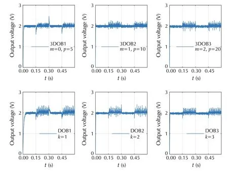
Fig. 10 Experimental results against load changes

Table 4 Closed-loop performance criteria against load changes

6.3.2 Case 2: Robustness against input voltage fluctuations

The second scenario test the robustness of the proposed strategy against input voltage variations. This test has special relevance in buck converters due its poor line rejection and because the control-to-output transfer function changes between operating modes. Likewise, the input voltage disturbance acts as a matched perturbation input in the input-output system model. During the test, the input voltage has smooth changes around its nominal value (Vin), with an amplitude of 22% and a frequency of 10 Hz, according to the following profile:

The experimental curves of the output voltage under the proposed 3DOB-based controller and the classical DOB are shown in Fig. 11. Moreover, the performances indices IAE,ISE, MAE and MSE are presented in Table 5.

According to the above experimental tests, although both 3DOB and classical DOB approaches are able to reject the mismatched disturbances caused by hard sudden load changes, the closed-loop performance is improved by the proposed 3DOB-based control as is shown in Table 4. Furthermore, the performance results in 3DOB further improves with a large polynomial order since the local approximation of the disturbance is better, even for smaller bandwidth.On the other hand, results presented in Fig. 11 and Table 4 show that the results of the two approaches are comparable; however, the proposed control strategy minimizes all criteria compared with the classical strategy in the case of input voltage fluctuations. Besides, significant improvements occur in 3DOB with polynomials with order greater than zero.

Finally, it is worth noting that according with practical implementation issues, such as noise and sampling period,it is possible to find different tuning rules for both the proposed data-driven disturbance observer and classical DOB and HODOB, which allow to achieve satisfactory performances. However, from the results obtained in this work, it is viable to conclude that the data-driven proposed approach is capable of achieving similar and even superior performances (under certain conditions) compared to another disturbance/uncertainty estimation and attenuation techniques,such as disturbance observer-based control (DOBC). Likewise, it is important to note that, the inherent phase lag isreduced in the disturbance observer mechanism, leading to potential for faster response, which is needed in applications like DC-DC converter.

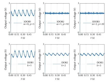
Fig. 11 Experimental results against input voltage fluctuations

Table 5 Closed-loop performance criteria against input voltage fluctuations

7 Conclusions

A data-driven disturbance observer-based control strategy with an active disturbance rejection approach is developed.The general control scheme is composed by two stages: first a inner stabilisation loop based on an unity feedback controller or a two parameters compensator is developed to set the desired closed-loop dynamics. Then to estimate and reject the equivalent disturbance in the outer loop, an observer that includes a prediction scheme, based on a least-square regression, is proposed.

A key feature of the proposed approach is its flexibility to select the design parameters, such as the polynomial orderm, and the number of samplespin the predictor. This feature allows to adjust the best performance and at the same time to reduce the effect of noise. Furthermore, the proposed predictor scheme fulfills the same effects of the classical-DOB, but without the explicit use of an inverse of the plant dynamics or the design of a digital Q-filter. Additionally, it is possible to use the frequency response analysis to help the parameter tuning and to achieve the desired performance.

In other matters, the proposed approach not only has a performance and a robustness comparable at least with those of another related methods, but also it presents a new point of view that takes advantage of the use of data. This aspect that could be considered as a superiority and an opportunity to open a line of research regarding the use of data-driven techniques in disturbance estimation and rejection schemes.

Finally, the robustness and performance of the proposed strategy is validated in a case study for the voltage control of a DC-DC synchronous buck converter affected by disturbances in the input voltage and the load. The experimental results show the data-driven disturbance observer-based control is able to reject matched and mismatched disturbances and the performance is improved in comparison to the classical disturbance observer-based control.