Simplifying ADRC design with error‑based framework: case study of a DC-DC buck power converter

Rafal Madonski · Krzysztof Łakomy · Jun Yang

Abstract

Keywords DC-DC converter · Power electronics · Active disturbance rejection control · ADRC · Extended state observer ·ESO · Error-based form

1 Introduction

The DC-DC converters of ‘buck’ type are important elements in the process of power conversion, responsible for stepping down voltage from its input (supply) to its output (load).Due to their high efficiency, compact size and low cost, buck converters find wide applicability in catering to essential DC voltage requirements for various types of loads. Their significance is especially noticeable now, with the major development of smart grids and exploitation of new sources of renewable energy such as photovoltaic and fuel cells.

To guarantee satisfactory performance of connected loads or devices, the task of controlling output voltage in the buck converter is of great importance. It is however problematic as buck converters are variable structure systems and inherently exhibit nonlinear, non-smooth, time-varying dynamics.The specific challenges in their control lie in the following aspects [1]: (i) modeling uncertainties related to unmodeled voltage drops across active and passive switches, parasitic capacitors associated with the switches, unmodeled sensor dynamics, nonlinear magnetic characteristics of inductor coil and time delays involved during switching action; (ii)sensitivity to frequent input voltage fluctuations due to unreliable supply; (iii) unknown load disturbances. Hence, the potential control algorithm for DC-DC converters has to be sufficiently robust against internal and external disturbances over a wide operating range to provide satisfactory results in transient and steady-state performances.

Some practically appealing results were recently achieved for buck converters with techniques based on the idea of active disturbance rejection control (ADRC, [2]). Owing to its disturbance-centric approach of solving control problems [3], the resultant governing principle in ADRC is powerful (yet relatively simple to grasp, implement, and commission), combing both adaptive and robust features.The detailed characteristics of the ADRC methodology has been described in latest survey papers [4-7]. The efficiency of ADRC methods has been validated by now in various experimental and industrial case studies, recently summarized in [8]. Its engineering proficiency has been confirmed by theoretical analyses, carried out in e.g., [9-14]. What is more, intuitiveness of ADRC in design and tuning as well as its track record of successful applications has attracted industry (e.g., Texas Instruments, Danfoss), that has now embedded this approach in some of its control solutions. As the ADRC emerges as a viable general solution for industrial control, research interests have been intensified in the area of power electronics devices. In the case of buck converters,considerable amount of works have been published in the last few years that proposed ADRC solutions (e.g., [15-18]).They address typical control tasks for DC-DC conversion(regulation, trajectory following), and tackle various specific problems occurring in them (fast-varying perturbations,mismatched disturbances) by using spectrum of tools (e.g.,sliding surfaces, finite-time observers, optimization through model reduction).

Motivated by the recent interest in ADRC in power electronics research, in this work, a practical simplification of the ADRC design is studied for the specific case of output voltage control in DC-DC buck power converter. In particular, a trajectory following problem in buck converter is considered,in which the reference trajectory cannot be preprogrammed,hence straightforwardly utilized in the control design. The simplifying solution is proposed in the form of a recently introduced error-based ADRC scheme (independently developed in [19, 20]), which takes advantage of expressing the control objective in alternative, feedback error domain. For this specific work, it means that the uncertainty related with the unavailability of higher-order reference trajectory signals for the buck converter can be treated as a source of an external disturbance, to be timely estimated and actively rejected by the means of a disturbance observer. Such approach significantly reduces the complexity of control structure as it makes the reference signal differentiators obsolete and trivializes the formulation of the outer compensation loop to simple proportional (static) output feedback controller, regardless of the system dynamics. In other words, the focus here isshiftedfrom the conventional trajectory following control design, with a tedious task of reconstructing reference derivatives with a differentiator, to the set-point tracking in the feedback error domain, where a disturbance observer is used to accurately and quickly reconstruct the resultant disturbance including the uncertainty related to unknown higher-order reference terms.The error-based ADRC has been successfully applied by now to a variety of control problems including mechanical vibration compensation [21, 22], robotic manipulator control [23,24], observer design with suppression of sensor noise [25-27],position control of a telescope mount [28], UAV control [29,30], as well as power electronics control [31, 32].

This article is an extended version of the work initially presented in [31]. In the light of existing literature, the contribution of this work is threefold.

1. Multi-criteria numerical and experimental evaluation of the error-based ADRC strategy for trajectory following task in DC-DC buck converter without the availability of reference time-derivatives.

2. Quantitative and qualitative comparison with conventional, output-based ADRC form.

3. Convergence and stability analysis of the error-based ADRC. In contrary to the already available stability proof of error-based ADRC from [32], here a more general form of the total disturbance is assumed and takes the form of a Taylor polynomial structure.

The rest of the paper is organized as follows. Some preliminary information about the plant model and the considered control objective is first given in Sect. 2. Section 3 recalls the conventional, output-based ADRC and shows its specific and general forms for the considered DC-DC buck power converter.Analogously, Sect. 4 recalls the error-based ADRC and also shows its specific and general forms for the buck converter.Section 5 contains information about the conducted numerical and experimental validation, including chosen methodology,description of the utilized laboratory testbed, and obtained results (followed by a discussion). Finally, Sect. 6 summarizes the work.

2 Preliminaries

2.1 Model of a DC-DC buck power converter

By referring to the Kirchhoff’s voltage and current laws, the dynamic model of a DC-DC buck converter system, illustratively depicted in Fig. 1, is given as

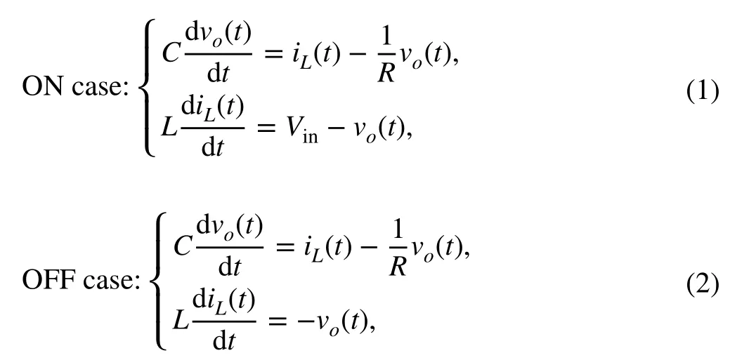
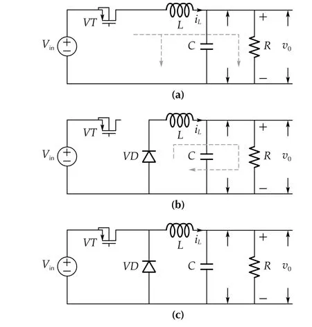
Fig. 1 Circuit diagram of the semiconductor realization of the considered DC-DC power converter of “buck” type, with diode VD and control switch VT, a ON case, b OFF case, c average case

where the above switching structure can be also expressed with a followingaveragemodel ([18]):

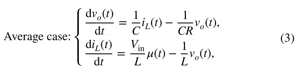
whereμ∈[0,1] is the duty ratio (control signal)1In the considered average model, it has replaced the discrete input μ ∈{0,1} , since PWM strategy is used here to generate governing signal from an analog input signal.,vo[V]is the average capacitor output voltage (controlled signal),iL[A] is the average inductor current,R[Ω ] is the load resistance of the circuit,L[H] is the filter inductance,C[F] is the filter capacitor, andVin[V] is the input DC voltage source.

Remark 1Even though the system mathematical model (3)is assumed linear,2Note that the linear system description is valid only as long as it can be ensured that no saturation effects occur in the coil. Otherwise,the inductance L would depend on the current iL nonlinearly.the amount of structural and parametric uncertainties (mentioned in Introduction), the likelihood of outside interferences (potentially of nonlinear nature), as well as the fact that analytical form ofvr(t) , its future values,and reference time-derivatives are not always available for control design purposes, makes this a nontrivial control task in practice. Due to the robustness of the ADRC framework,such simplified system description will be used nevertheless throughout the work to simplify the control algorithm synthesis.

2.2 Control objective

In this work, a trajectory following task is considered with a reference average capacitor output voltage being defined asvr(t) [V]∈ℝ+and satisfying following assumptions:

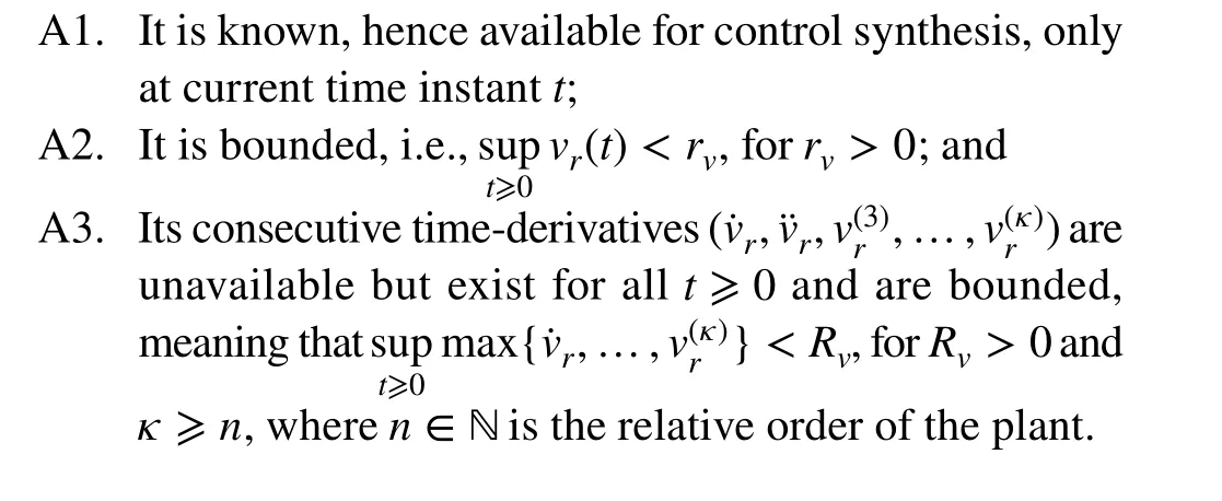
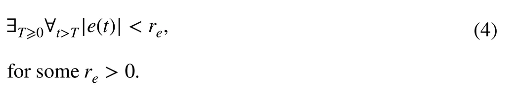
The control objective is to force the average capacitor output voltagevo(t) to follow the desired trajectoryvr(t) by manipulating the duty ratioμ(t) , in spite the presence of various uncertainties, represented, e.g., by load resistance changes(R0≠R)3Subscript “0” represents the nominal value of the parameter., input voltage variations (Vin0≠Vin), circuit parametric variations (L0≠L,C0≠C), external interferences, as well as unavailability of target time-derivatives A3. Assuming practicality of the desired result, the controllerμ(t) has to make the absolute trajectory-following error|e(t)|≜|vr(t)-vo(t)| ultimately bounded by some small (but practically acceptable) numberψ, meaning that

3 Output‑based ADRC

3.1 General form

In the conventional output-based ADRC, as seen in [11],modeling of a highly disturbed buck converter would come down to representing it with some variation of a following input-output model,4Notation of signals dependence (on time, on states, etc.) will be omitted here and throughout the paper for presentation clearance(e.g., v(t,x)=∶v(·)=∶v ) with exception of instants when specification is notably important for the considered context.describing generalnth order controlaffine system disturbed by a matchedtotal disturbanceF(·):

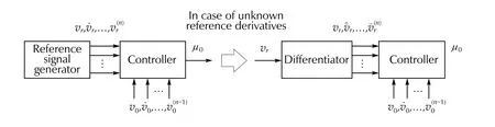
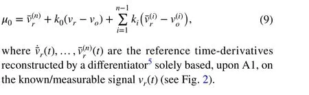
Fig. 2 An illustrative example of using a differentiator as a potential solution in case of needed, but unavailable, timederivatives of the target signal

wherepstands for the overall parametric uncertainty,f(·)∈ℝ encapsulates external disturbances and unknown(or uncertain) parts of the system that cannot be accurately expressed with a mathematical model or physically measured, andb≠0 represents the uncertain input gain (also denoted ascritical gain parameter, or CGP [33]) with≠0 being its available approximation.

In the considered output-based ADRC framework, when defining a trajectory following objective for system (3) (withvr(t) being a sufficiently smooth reference signal), one usually proposes a following conventional two-step procedure to realize it. The first step is the construction of an inner,disturbance compensation loop:

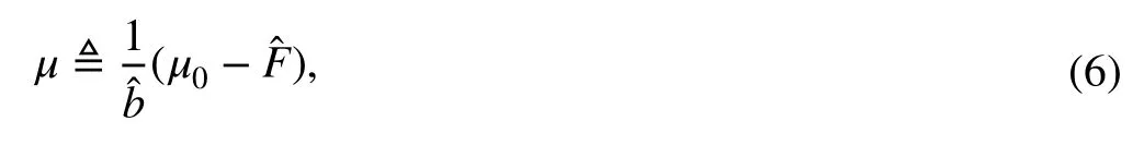
forrepresenting the estimate oftotal disturbance. The second step is achieving robust feedback-linearization of the original system dynamics through designing an outer control loop for the (theoretically) disturbance-free model of chain of integrators. This is often realized through a standard output-feedback controller in the form of

3.2 Stability analysis

The stability of the conventional output-based ADRC has been well-documented by now in e.g., [9-14], hence will not be studied in details here. For example, through a singular perturbation analysis shown in [11], a uniform asymptotic solution can be obtained for the above standard ADRC closed-loop system and an exponential stability in the error dynamics can be established under the condition that the initial observer error is reasonably small. The result holds under a mild condition oftotal disturbancedifferentiability w.r.t. timet.

3.3 Specific form for DC-DC buck power converter

3.3.1 Expressing control task in output domain

Following the standard ADRC line of reasoning from [11],the plant model from (3) can be first reformulated, assumingn=2 , as

which forms a desirable, integral chain system perturbed solely with a matchedtotal disturbanceF(·).

3.3.2 Disturbance observer design and tuning

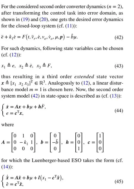
To design the controller in form of (6) for system (11),the focus now is on precise and on-line estimation of the perturbing termF(·) , crucial for further properactivedisturbance rejection. Hence, for the second order system model (11), state variables can be first chosen as

thus resulting in a third orderextendedstate vectorx≜[x1x2x3]T∈ℝ3, where the augmented state variable represents solely the lumped, additivetotal disturbance. At this point, additional assumption is introduced:

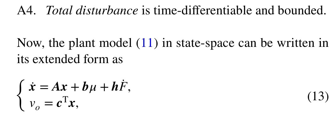
where

For such fully observable system, one can now propose a disturbance observer to reconstruct the information about state vector, including thetotal disturbancepart. One can choose from a spectrum of techniques, surveys of which can be found in [6, 28]. Here, and in this work in general, a linear Luenberger-like extended state observer (ESO) is used for its relatively high effectiveness-to-complexity ratio. For the considered case (13), it takes the form:

3.3.3 Control rule design and tuning

The control signal (15) applied to the considered system model (11) gives

Fig. 3 Output-based ADRC approach for the trajectory following task of the DC-DC buck converter without the availability of reference time-derivatives

Remark 2One can notice, based on (16), that for the proper realization of the control task, the speed and precision of not only state variables estimation (by ESO), but also signals reconstruction (by TD), is of crucial importance to the stability of the system. This additionally motivated to develop techniques, like error-based ADRC, that would minimize(desirably eliminate entirely) the role of the differentiator.

3.3.4 Reconstruction of reference time‑derivatives

To propose a control rule for the considered buck converter (11) in form of (9), one needs to provide two consecutive time-derivatives of the reference signal. Here, a TD is used, which produces an estimate of the target timederivative on-line by continuously solving the following set of equations:

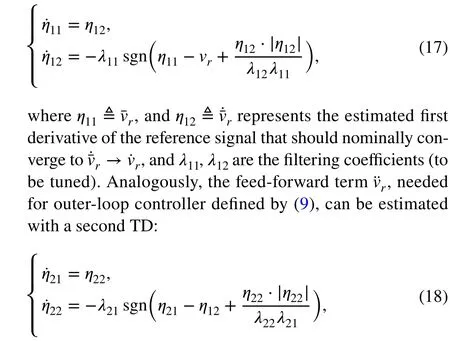
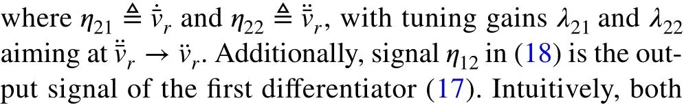
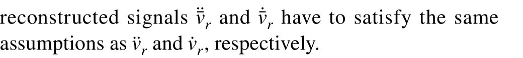
However introducing a differentiator in the control structure results in an additional element that has to be physically implemented and tuned. Such extra complexity, especially for higher order plant models, could be discouraging from an engineering viewpoint, which favors design swiftness and compactness. Another problem is the increased difficulty of theoretical analysis of the closed-loop system containing a differentiator,as discussed in [35]. It was thus desirable to pursue an alternative way, which would address the problem of unavailability of time derivatives of the target signal, while retaining not only the capabilities and intuitiveness of the output-based ADRC,but also its structure conciseness. Hence, the error-based modification of ADRC was developed in [19, 20] and its design for the considered buck converter is shown next.

4 Error‑based ADRC

4.1 General form

To address the above concerns related to the availability of time-derivatives of the reference signal, one can find a potential solution in recently published works proposing the error-based ADRC [19, 20]. Certain parts of these works will be revisited first for completeness and to retain the train of thought. The error-based approach will be explained for general type systems as this form will be later useful for the theoretical analysis. Subsequent section will contain a specific application to the considered buck converter control problem.

4.1.1 Expressing control task in error domain

Recalling the trajectory-following errore(t)≜vr(t)-vo(t) ,one can write

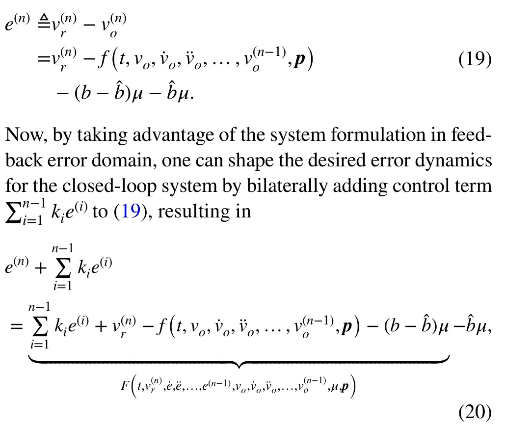
whereki ＞0 are design control coefficients (to be selected)andF(·) is thetotal disturbancedefined in error-domain (cf.(5)), to be reconstructed and then timely rejected.

By reformulating the control task in the error domain, the objective now is to stabilize the new output signaleat zero with the use of same control inputμ, despite the influence of (matched) disturbanceF(·) . In other words, by the above reformulation of the standard ADRC, assumption about the availability of the reference time-derivatives, that limited the outer-loop control action [both the generic one (7) and the specific one (15)] has been removed entirely. What is important, is that the perturbing effect of unknown time-derivatives of the reference signal is treated as part of thetotal disturbanceF(·) , which makes the differentiator obsolete.

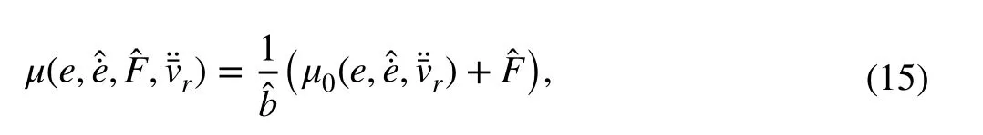
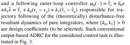
4.1.2 Control rule design and tuning

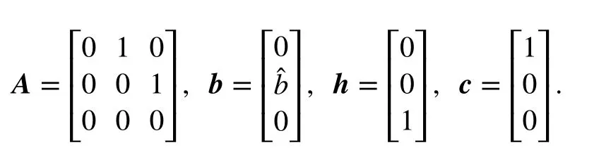
Now, assumingF(·) from (20) is accurately reconstructed with the ESO (i.e.,≡F), one can propose a following governing action:

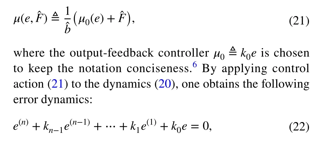
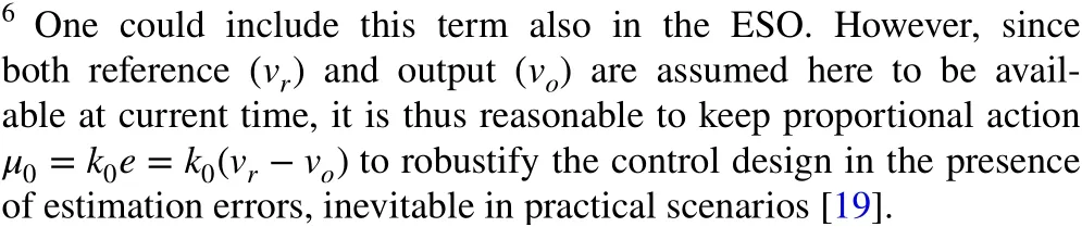
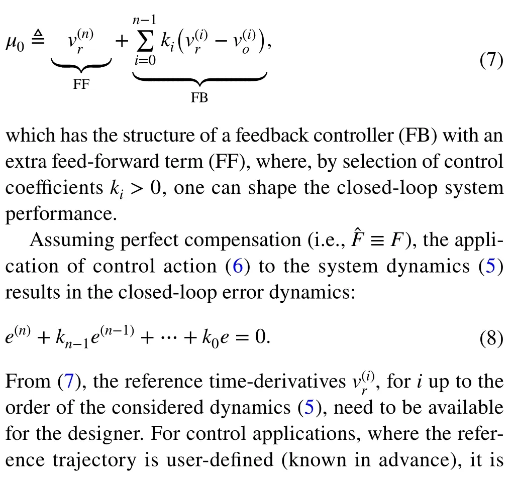
which determines the prescribed control behavior of the resultant (theoretically) disturbance-free chain of integrators, in accordance to gainski ＞0 , fori=0,…,n-1.

Still assuming perfect uncertainty cancellation (i.e.,≡F), same popular and effective parametric synthesis of the controller based on pole-placement approach [35],known from the conventional ADRC tuning, can be used here as well. It is based on defining a frequencyωc ＞0 ,which determines the desired bandwidthΩc=[0,ωc] of the closed-loop system. Comparison of the characteristic polynomial of dynamics (22) with a desired polynomial(s+ωc)n:

which places all the poles at one location -ωc, greatly simplifies the tuning process, as it is reduced to a single parameter selection (ωc) for controller coefficients computation.Some general forms of the controller gains for thenth order plant model parametrized byωcare gathered in Table 1.

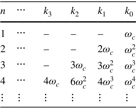
Table 1 General forms of controller gains for nth order plant model parametrized by frequency ωc (here for n={1,2,3,4})

4.1.3 Disturbance observer design and tuning

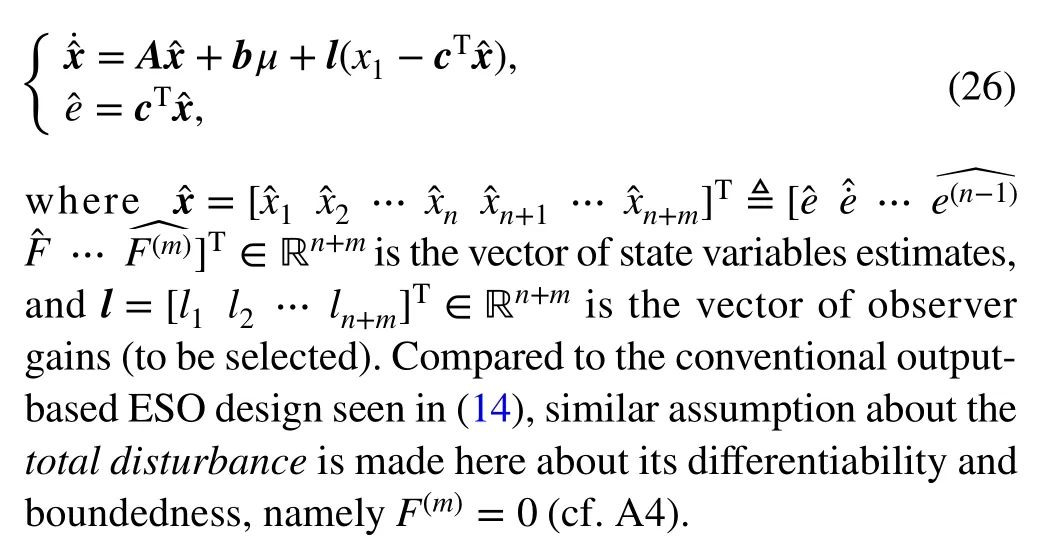
In contrary to the source material [19, 20], in which (n+1) th order ESO has been used, here a higher-order observer is utilized, which further generalizes the result. The theoretical analysis is also conducted using the proposed more general,higher-order ESO (see Sect. 4.2).

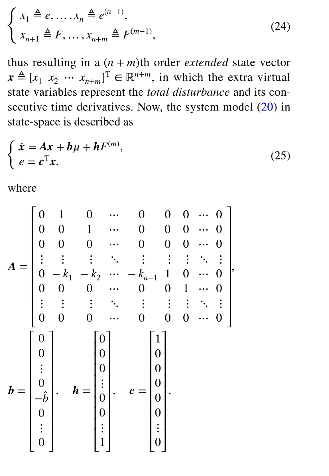
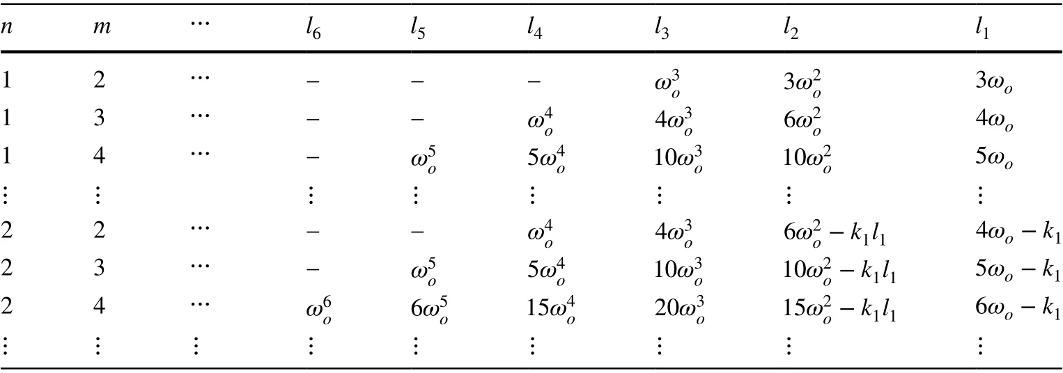
Table 2 General forms of(n+m) th order ESO gains parametrized by frequency ωo (here for n={1,2} and m={2,3,4})

For thenth order dynamics (20), a following set of state variables can be chosen:Since the system (25) is observable, one can propose a following (n+m) th order ESO (also known as generalized proportional integral observer, or GPIO [36]) to estimate its states, which similarly to the observer (14) in the conventional ADRC design, only uses practically available plant input and output signals:

It is notable that the prescribed error dynamics (22) isincorporatedinto the ESO structure (with the exception ofk0), making the state matrixAdependent on the design coefficientsk0,…,kn-1. This trivializes the outer-loop controller as it is reduced in (21) to just a proportional outputerror feedback action, regardless of the order of the system dynamics. That feature is especially appealing to practitioners as it simplifies the control, compared to conventional ADRC design, where the outer loop requires the availability of the reference time-derivatives up to the order of dynamics(see (15)).

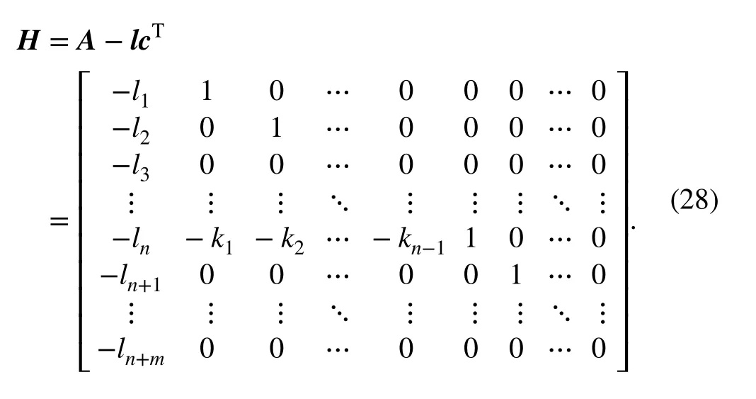
The pole-placement technique for observer gains parametrization, known from the conventional ADRC design,can be used for the error-domain system as well. The goal is to place the roots of characteristic polynomial det(λI-H) in the complex plane (desirably far) on the left-hand side of the roots determined for corresponding system representations in Sect. 4.1.2. Following previous results related to ESO tuning [35], it can be effectively done by forcing

whereωois a design frequency that determines the observer bandwidthΩo=[0,ωo] and the estimation-error state matrix has the form:

Some general forms of the observer gains for the (n+m) th order plant model parametrized by frequencyωoare gathered in Table 2. The stability proof of the above observer is given in Sect. 4.2. Next, the above general approach will be applied to the specific problem of controlling the DC-DC buck converter.

4.2 Stability analysis

The stability of the considered error-based ADRC [19, 20] is proved here using the singular perturbation method [37]. The analysis is thus divided into “fast” observer part (Theorem 1)and “slow” controller part (Theorem 2). The performed analysis is a modification of the stability proof of output-based ADRC given in [38]. In contrary to the already available stability proof of error-based ADRC from [32], here a more general form of thetotal disturbanceis assumed and takes the form of a Taylor polynomial structure (see (24)).

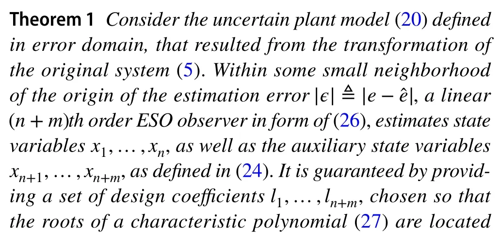
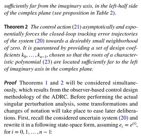
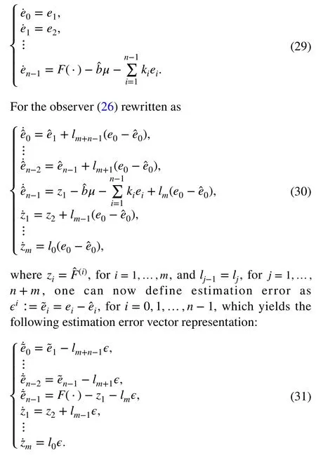
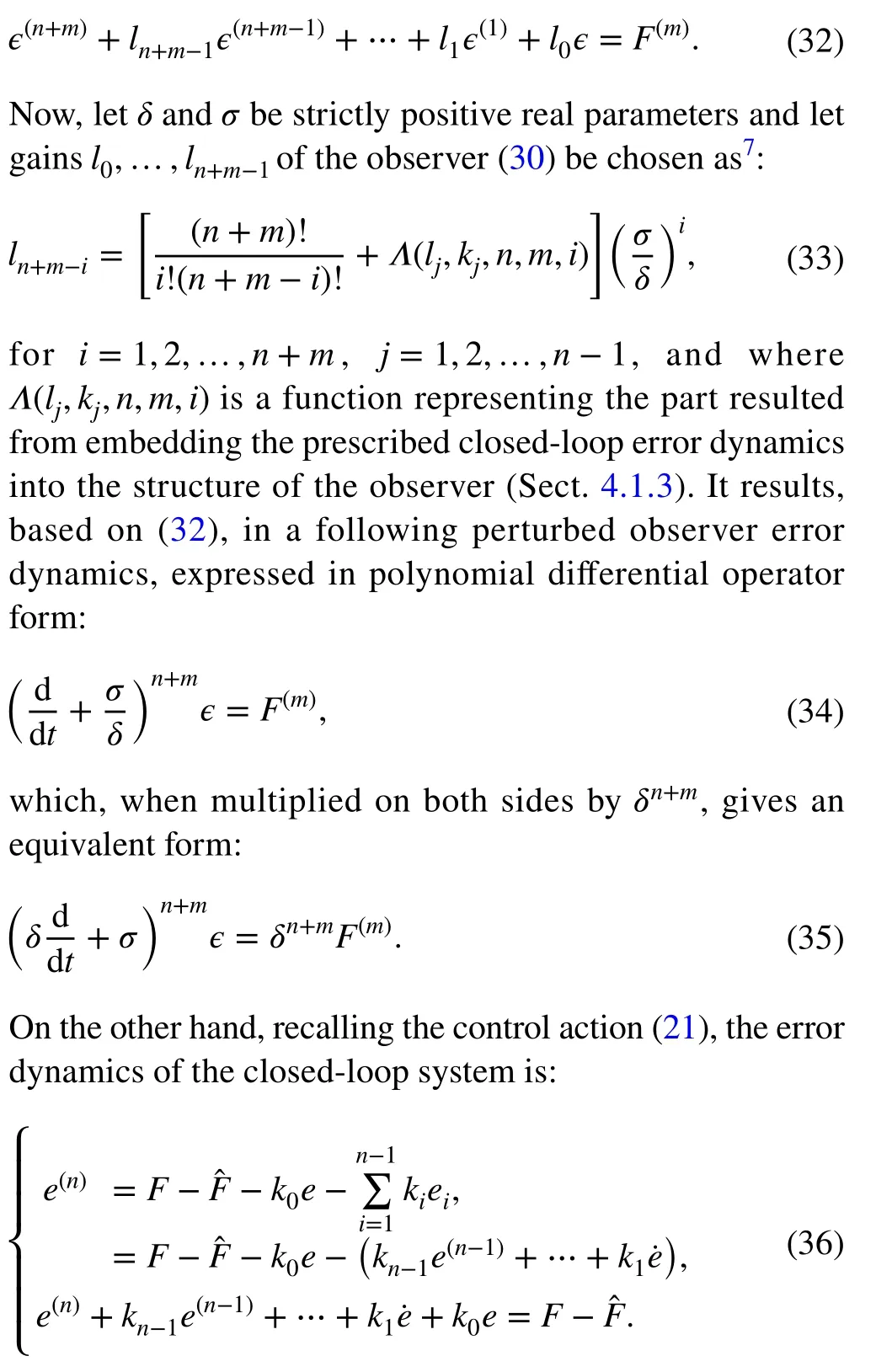
Based on the above, the estimation error∈∶==e0-satisfies the following perturbed (n+m) th order differential equation:

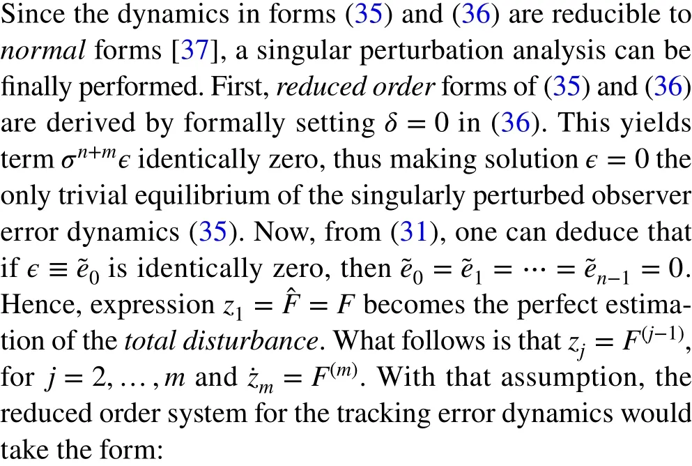
which, for the made assumptions on the controller parameters (Sect. 4.1.2), has the origin as an asymptotically, exponentially stable equilibrium point.

Following work [38], the corresponding boundary layer system, described in a stretched time scaleτ=t∕δ, and denoted by the correction variableez=∈-0=∈, satisfies an asymptotically stable linear homogenous differential equation:

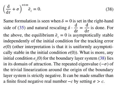
By definingKmas the uniform absolute bound, hypothesized onF(m), the estimate of the radius of an ultimately uniformly bonding open neighborhood for∈can be expressed as (δ∕σ)(n+m)Km(it is thus intuitive thatσshould be chosen larger than one). Let recall from (31) that of if allwere not identically zero, but ultimately uniformly arbitrary close to zero, thenz1≈Fwould also be an ultimately arbitrary close estimate of thetotal disturbance(this justified the notationz1=in the first place). Hence, the differenceF-z1is also arbitrary small and the estimation of thetotal disturbancecan be made desirably small (at least theoretically),by manipulatingσandδ.

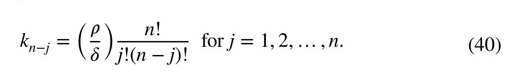
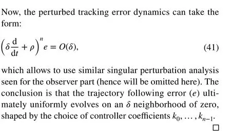
On the other hand, the controller coefficientsk0,…,kn-1are chosen using the same pole-placement-based approach as seen in Sect. 4.1.2, hence for a finite positive real numberρ ＞0:

4.3 Specific form for DC-DC buck power converter

One can now directly apply the following governing action, without the need of a differentiator (cf. (15)):

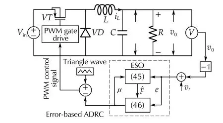
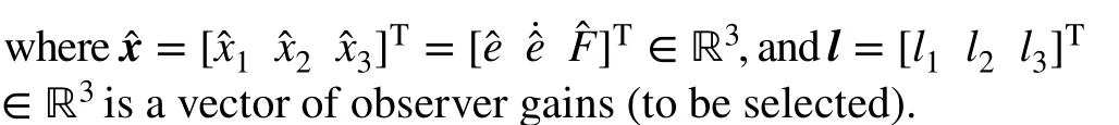
Fig. 4 Error-based ADRC approach for the trajectory following task of the DC-DC buck converter without the availability of reference time-derivatives (cf. Fig. 3)

The ADRC-based approach for the trajectory following task of the DC-DC buck converter without the availability of reference time-derivatives is depicted in Fig. 4. Validation of the error-based ADRC, including its comparison with output-based ADRC, is presented next.

5 Numerical and experimental validation

5.1 Methodology

To further study the error-based ADRC for the considered DC-DC buck power converter, several numerical and experimental tests are conducted (see Table 3). The use of both simulation and experiment is justified here by the fact that some of the planned numerical tests aim at verifying the intrinsic capabilities of the utilized control in idealized scenarios, whereas conducted experiments test its practical usefulness.

The task in both simulation and hardware tests is to follow desired average capacitor output voltage trajectory(Sect. 2.2), that satisfies assumptions A1-A3 and is in form ofvr(t)=H(s)[v*r(t)] , wherev*r(t) is a rectangular signal(with amplitudeAand time periodT) filtered by a linear,stable dynamicsH(s). This imitates a scenario, in whichvr(t) is a response of some external, unknown dynamical system, thus implying the unavailability of reference timederivatives at any given time. In the conducted study, the parameters of the target signal are selected asA=50 V,

T=1 s, andH(s)=4∕(0.025s2+0.6s+4).

For the considered second order plant (n=2 ) and assumed first order disturbance model (m=1 ), a third order observer is chosen as thenominalcase. The initial conditions for all the considered signals are set to zero. The nominal tuning parameters of the used scheme in both simulations and experiments areωc=130 andωo=65×102,which according to the chosen parametrization techniques(described in Sects. 4.1.2 and 4.1.3 for the controller and observer part, respectively) givesl1=19240 ,l2=12174.76×104,l3=27463×108for the observer part,andk0=16900 ,k1=260 for the controller part. The tuning of observer and controller bandwidths (ωoandωc) is performed manually based on guidelines from [35], and aim at a practical compromise between estimation/control accuracy and noise amplification. It also comes from a simple reasoning that the closed-loop error dynamics can be naturally separated into two kinds: fast observer dynamics (shaped byωo) and slower dynamics of the feedback loop (shaped byωc), which additionally suggests thatω0≫ωc.

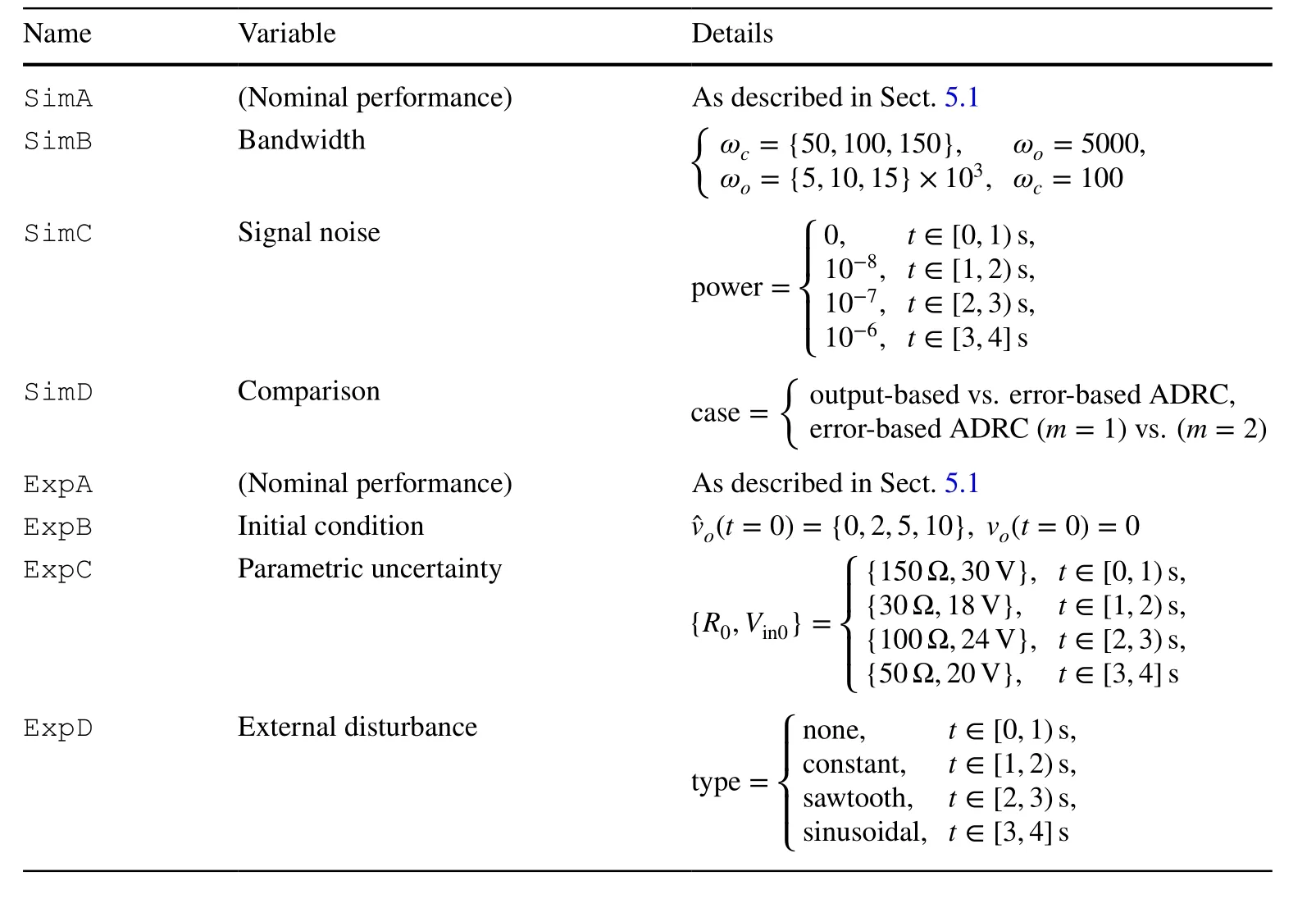
Table 3 Conducted simulation(Sim) and experimental (Exp)tests

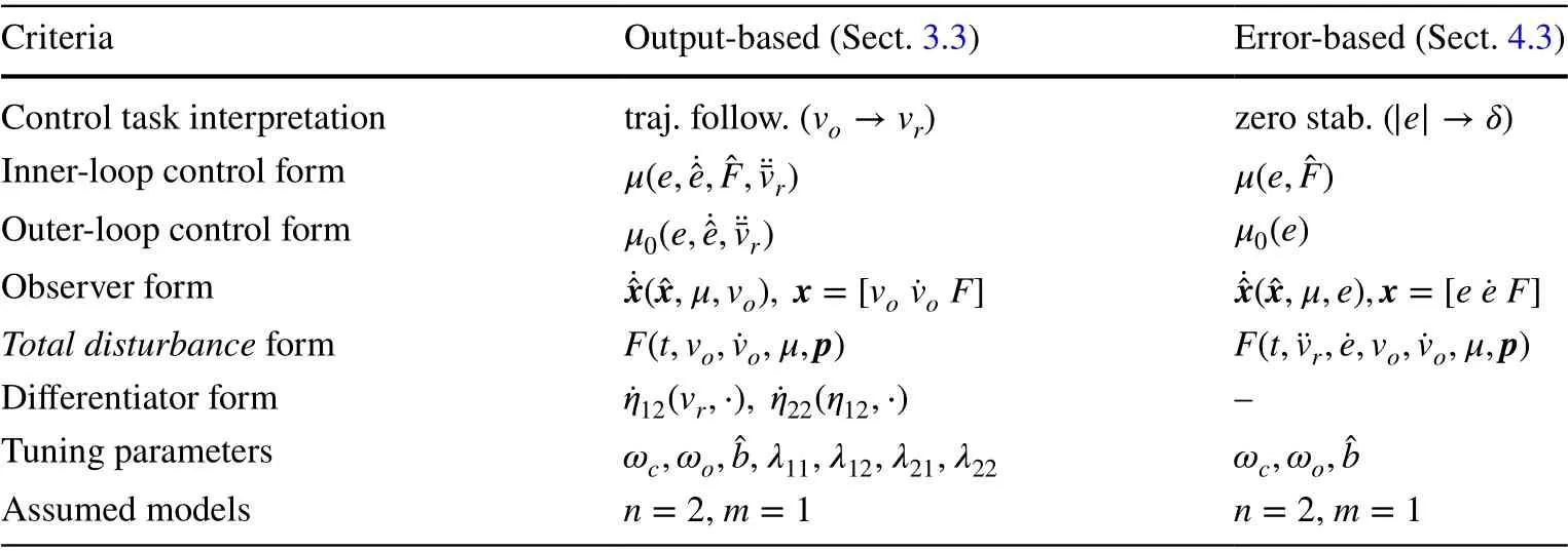
Table 4 Comparison between specific forms of output- and error-based ADRCs for buck converter trajectory tracking in terms of control design complexity

One of the planned test (SimD) is a comparison between the conventional output-based ADRC (Sect. 3) and its error-based version (Sect. 4). Based on Table 4, however,which shows their relative design complexity, comparison of these two approaches, that have different: interpretation of the control task, amount of assumed uncertainty, observer and controller structures, number of design parameters, and essentially different influence of particular parameters on the dynamic and static quality of control process, may not give reliable results. Conclusions made from such analysis may be too far-reaching or even untrue in general case. Nevertheless, some careful forms of comparison (one is made in Table 4) will be carried out here, which is justified by the fact that the considered error-based ADRC originates from the classic output-based ADRC and realizes the same control goal, hence naturally bares similarities.

An example of a subjective and heuristic evaluation in regards to standard ADRC scheme, based on selected criteria, is depicted in Fig. 5.

5.2 Laboratory setup

An open-loop comparison between the actual system and its assumed analytical description is seen in Fig. 7.

5.3 Results

The considered error-based ADRC for buck converter is tested first in a Matlab/Simulink simulation environment.The entire control system is implemented in continuous form with sampling frequency resembling that of the experiment(i.e.,fsim=fexp=10 kHz) with a fixed-step size solver (type ODE1). Except dedicated test SimC, no noise is assumed in the numerical tests. In case of the quantitative comparison with the conventional, output-based ADRC (SimD), the tuning gains for the TD (described in Sect. 3.3.4) are selected asλ11=3×104,λ12=9×104(for TD estimating first reference time-derivative), andλ21=9×105,λ22=18×105(for TD estimating second reference time-derivative). The differentiators tuning is performed heuristically following guidelines from [2], aiming at a practical compromise between speed of reconstruction, its precision, and sensitivity to uncertainties. The results of numerical tests SimASimD are presented in Figs. 8, 9, 10, 11, 12, 13, 14, 15, 16,17, 18, 19 and 20.

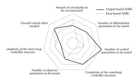
Fig. 5 Comparison of output-based and error-based ADRC (subjective and heuristic evaluation based on selected criteria)

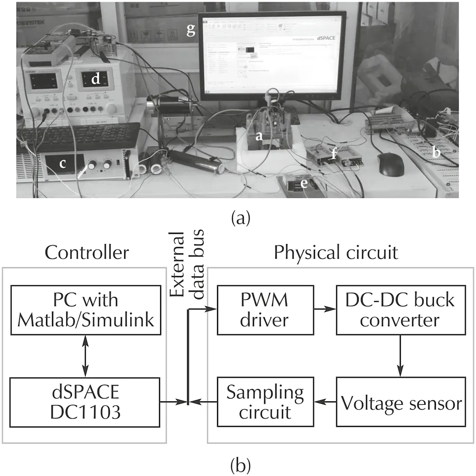
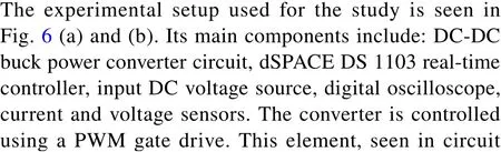
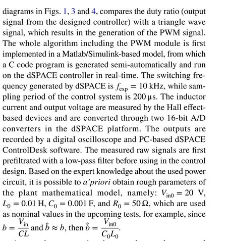
Fig. 6 Laboratory setup used in the experiments, with a - buck converter circuit, b - dSpace DS 1103 real-time controller, c - DC input voltage, d - digital oscilloscope, e - voltage and currents sensors, f- A/D converters, and g - PC-based dSpace ControlDesk software. a Hardware overview. b Hardware configuration

The outcomes of SimA, depicted in Figs. 8, 9, 10 and 11,present the nominal performance of the buck converter in trajectory tracking task with the error-based ADRC. Both the tracking error (Fig. 9) and the estimation error (Fig. 10),are kept within satisfying margins, even with the amount of simplifications introduced at the design stage (Sect. 4.1.1).What is important, the governing signal (Fig. 11) and the inductor current (Fig. 12) do not exceed the permissible saturation level. These results serve as a nominal case, which is a base for further tests.

Test SimB investigates the influence of observer and controller desired bandwidths on the performance of the closedloop system. In Fig. 13, one can see that (intuitively) with the increase of the control bandwidth, the amplitude of the absolute tracking error is decreased. Analogously, in Fig. 14,with the increase of the observer bandwidth, the amplitude of the absolute estimation error is decreased. These two intuitive relations are retained from the conventional ADRC.

The influence of measurement noise (here: band-limited white noise) on the estimation process, and consequently on the entire trajectory tracking is studied in SimC for two cases: when noise is present in the system output (Fig. 15)or in the reference signal (Fig. 16)8This emulates a scenario where the target signal comes from an outer-loop (i.e., cascade control) or from an entirely different, outside system.. This additionally shows that in the presence of measurement noise, the choice of observer and controller bandwidths is limited and is related with convergence speed to noise amplification ratio(cf. SimB).

The last numerical test SimD is a quantitative comparison with the conventional, output-based ADRC in terms of trajectory tracking (Fig. 17) and states reconstruction quality(Fig. 18). One can notice that the error-based ADRC with its highly simplified control design realizes the trajectory following task without loss of performance. The Reader,however, is advised not to treat the results of such quantitative comparison as authors’ claim about the superiority of the error-based ADRC in terms of control accuracy, since the methodology for comparison was to set same observer/controller bandwidths, even for different observer/controller structures ]for example compare (14) with (45) and (15)with (46)]. Figures 19 and 20 present tracking and estimation errors, respectively, for the nominal case (m=1 ) and when a higher-order ESO is used instead (m=2 ). A significant quantitative reduction can be noticed in the case of assumed more complex disturbance model, although it should be noted that it results from larger values of observer gains(due to observer tuning methodology seen in Sect. 4.1.3).Same reason makes this observer more susceptible to signal noise (cf. SimC), thus in practice a compromise would be needed while choosingmandωo.

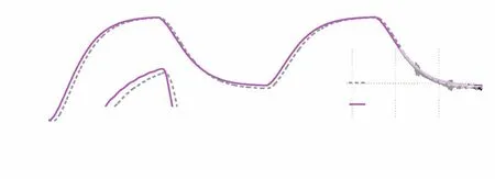
Fig. 7 An open-loop comparison between the actual system (before and after filtration) and its obtained mathematical model

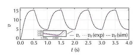
Fig. 8 [SimA/ExpA] Trajectory tracking in the nominal case

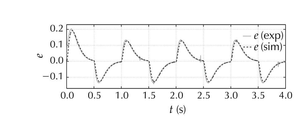
Fig. 9 [SimA/ExpA] Tracking error in the nominal case

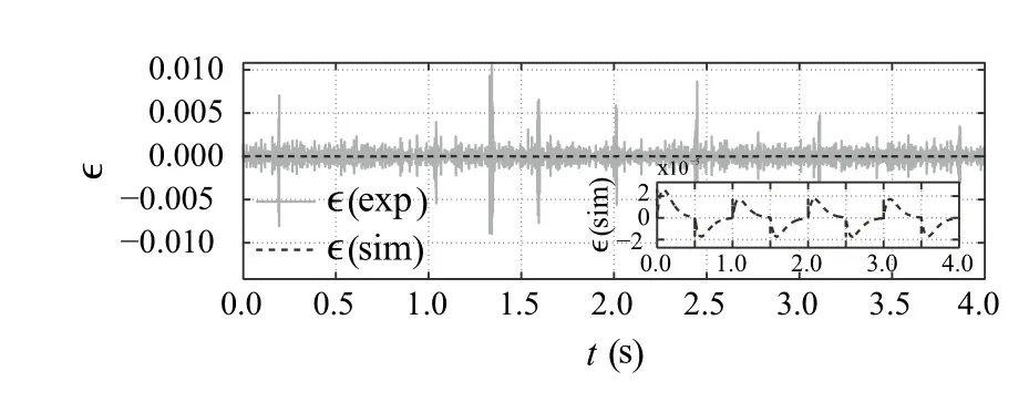
Fig. 10 [SimA/ExpA] Estimation error in the nominal case

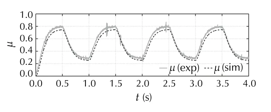
Fig. 11 [SimA/ExpA] Control effort in the nominal case

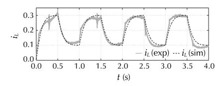
Fig. 12 [SimA/ExpA] Inductor current in the nominal case

Fig. 13 [SimB] Absolute tracking error for different controller bandwidths ( ωc ) and fixed observer bandwidth ωo =5000 (in log.scale)

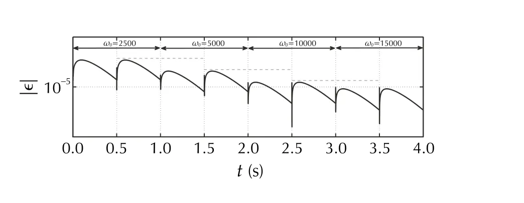
Fig. 14 [SimB] Absolute estimation error for different controller bandwidths ( ωo ) and fixed observer bandwidth ωc =100 (in log.scale)

Fig. 15 [SimC] Tracking and estimation errors for noisy output signal

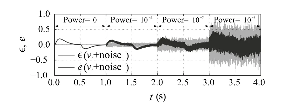
Fig. 16 [SimC] Tracking and estimation errors for noisy reference signal

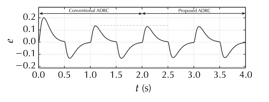
Fig. 17 [SimD] Tracking error of conventional and error-based ADRC

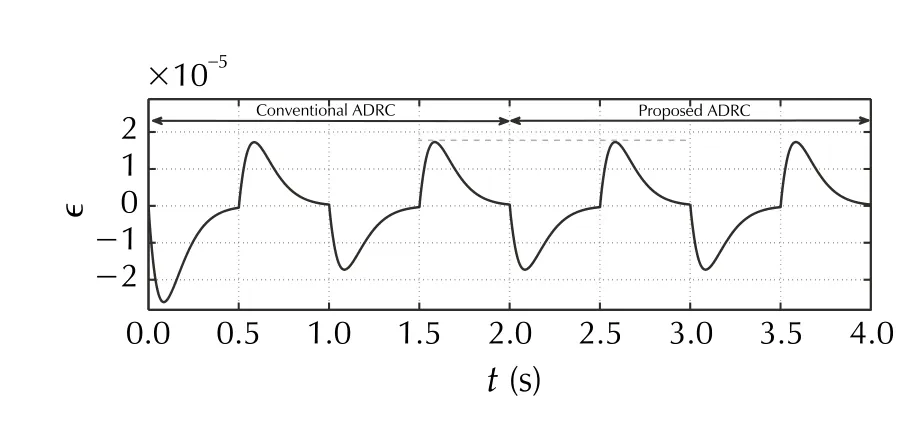
Fig. 18 [SimD] Estimation error of conventional and error-based ADRC

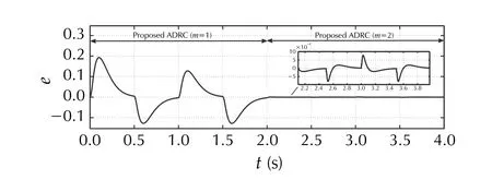
Fig. 19 [SimD] Tracking error of error-based ADRC for m={1,2}

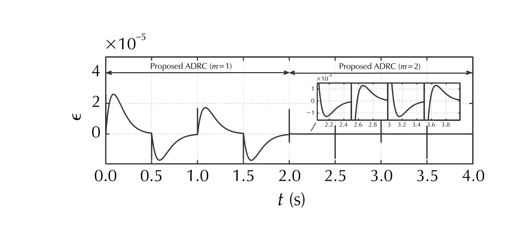
Fig. 20 [SimD] Estimation error of error-based ADRC for m={1,2}

The outcomes of the experimental tests ExpA-ExpD are depicted in Fig. 21, 22, 23, 24, 25, 26 and 27, with an exception of the nominal performance (ExpA), which is presented alongside analogous simulation result (SimA)in Figs. 8 to 12. The nominal behavior in hardware test is similar to the simulated one, providing an acceptable level of both estimation and control quality with the chosen tuning gains. In ExpB, the performance of the error-based ADRC is studied for various initial conditions (i.e.,(t=0)≠vo(t=0) ). One can notice in Fig. 21 that, after a short transient stage (less than 0.15 s) needed for observer convergence, the given task is realized as in the nominal case (i.e.,0)=vo(0)=0 ). Figures 22 and 23 are the outcomes of test ExpC, showing parametric robustness of the error-based ADRC for different values ofR0andVin0, respectively. The varying of both parameters has been obtained by physical changes made in the circuit.Checking robustness against uncertainty in parameterVinis at the same time a verification of robustness against parametric discrepancy in the input gain. One can notice that the introduced significant uncertainty did not largely changed the control performance (in terms of tracking error amplitude). The last test ExpD verified the robustness against external interferences affecting the system,according to a preprogrammed, user-defined sequence of disturbing signals seen in Fig. 24. The external disturbances were artificially added to the process in form of additive-input signal. Despite their interaction, the control performance remained at similar, acceptable level, as verified in Figs. 25 and 27.

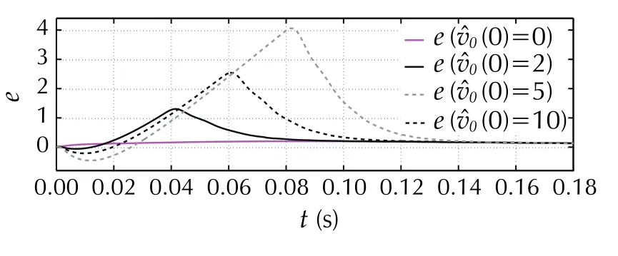
Fig. 21 [ExpB] Tracking error for different initial conditions(zoomed in)

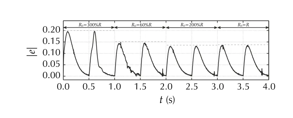
Fig. 22 [ExpC] Absolute tracking error for different load resistances R0

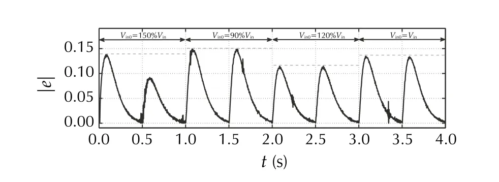
Fig. 23 [ExpC] Absolute tracking error for different input voltage Vin

5.4 Discussion

Analyzing the structure, characteristics, as well as obtained numerical and experimental results of the error-based ADRC for buck converter in trajectory following tasks without the availability of reference time-derivatives, one can draw following conclusions.

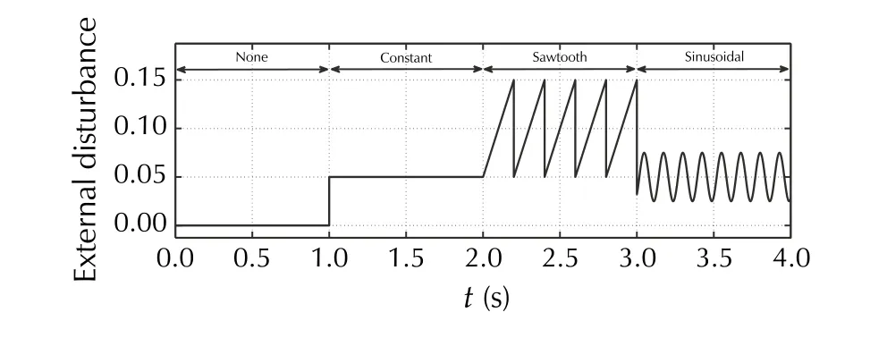
Fig. 24 [ExpD] Sequence of the user-defined external disturbance signal

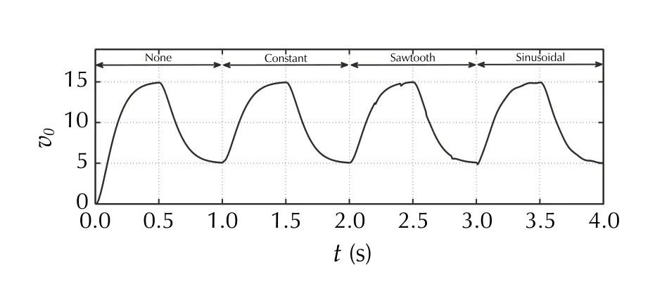
Fig. 25 [ExpD] Trajectory tracking in case of acting external perturbation

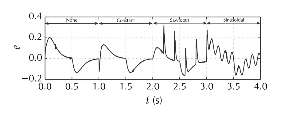
Fig. 26 [ExpD] Tracking error in case of acting external perturbation

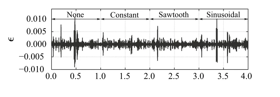
Fig. 27 [ExpD] Estimation error for different external disturbances

(a) The problem of unavailability of the reference timederivatives is shifted in the error-based ADRC from the problem of designing, implementing, and tuning a differentiator, to the problem of disturbance estimation and rejection. Thetotal disturbancereconstruction in the error-based ADRC however is additionally burdened with the uncertainty being the result of inclusion of unknown reference time-derivatives effect.That is the price for allowing a trivialized structure of the outer-loop controller and making differentiator unnecessary. Similar to the conventional output-based ADRC, the ESO remains the key element in the errorbased ADRC structure and its attentive construction and tuning is of crucial importance. What is especially important from practical perspective, the error-based modification of ADRC, compared to the standard output-based version, does not require any additional signals to be available or measurable.

(b) Results of tests ExpB and ExpC showed robustness and adaptability of the error-based ADRC, which the conventional output-based ADRC is known from.Additionally from ExpD, one can conclude about the capability of the error-based design in dealing with various types of disturbances. It is seen that for disturbance more complex than constant and piecewise linear ones, the estimation error, and consequently tracking error, do not converge to zero as seen int∈[2,4) , but rather to its neighborhood with its size being a function of observer/controller bandwidth). That is justified by the made assumption about thetotal disturbance(see A4).

(c) Even though the output-based and error-based ADRC schemes do not share the same structure, similar relations of the observer and controller with their respective bandwidths can be reported (see SimB and SimC).In the error-based version, analogously to typical errorbased ADRC, the selection ofωoandωcin practice should result from a compromise between some desired decay-time and factors like measurement noise, limited sampling frequency, and limited admissible amplitude of the control signal [35]. Since the disturbance rejection is not ideal in uncertain environments, the estimation error |∈| , and consequently the trajectory-following error |e|, are only ultimately bounded if bandwidth of the ESO is finite [13, 14]. It is also clear for this proposition, that the measurement noise and limited sampling remain the important factors in designing ADRC techniques in practice.

(d) The scalability of ADRC scheme is retained in its error-based modification as one can easily change the observer from linear ESO (26) to a different one to address certain disadvantages of current design (like the limited disturbance reconstruction capabilities seen in ExpD and its potential remedy in SimD in form of inclusion of higher-order disturbance model). Further improvement in quality could also be possibly obtained by modifications in the controller and/or observer structure (e.g., utilization of noise suppressing observers [25, 26] or reduced-order observers [18]).

(e) The core idea of ADRC is kept in its error-based version, since it still uses an elegant and effective way of canceling the complications from the uncertain dynamics and external disturbances, forcing the plant to behave like the ideal, chained pure integrators.

(f) Although tested in this work for a buck converter, the error-based ADRC retains the robustness of the conventional output-based design hence seems suitable for other types of power converters like boost and uk type, which, in general, exhibit more nonlinear behavior [36].

(g) Establishing a fair base and criteria for possible comparison (quantitative and qualitative) of the error-based ADRC with other methods (including output-based ADRC) remains an open issue.

6 Summary

The error-based ADRC has been successfully applied to the DC-DC buck power converter and comprehensively tested.It has been shown that in cases where the reference voltage trajectory cannot be preprogrammed, hence straightforwardly utilized in the control design, its higher-order terms can be treated (under some assumptions) as part of the lumped system disturbance. The uncertainty related to the unavailability of target time-derivatives can be thus shifted from the outer-loop controller design problem to the disturbance observer design problem, which corresponds with the fundamental disturbance-centric idea of ADRC.This allowed to introduce a custom robust control scheme for buck converter with following characteristics: (1) differentiator for reference signal is not needed; (2) just a proportional action in the outer loop is sufficient to stabilize the entire plant; (3)total disturbanceis effectively compensated without sacrificing the nominal performance despite major simplifications in the control design; and (4) tuning intuitiveness is retained from the conventional output-based ADRC approach.

AcknowledgementsThis work was supported by the Fundamental Research Funds for the Central Universities (No. 21620335).