Behavior recognition based on the fusion of 3D-BN-VGG and LSTM network

Wu Jin (吴 进), Min Yu, Shi Qianwen, Zhang Weihua, Zhao Bo

(School of Electronic and Engineering, Xi’an University of Posts and Telecommunications, Xi’an 710121, P.R.China)

Abstract

Key words: behavior recognition, deep learning, 3 dimensional batch normalization visual geometry group (3D-BN-VGG), long short-term memory (LSTM) network

0 Introduction

Video-based behavior recognition is an important application scenario in the field of computer vision. The study of behavioral recognition began in 1973 when the Swedish psychologist Johansson[1]proposed a model of moving light displays (MLD) that describes human motion behavior. It is widely applied in intelligent security monitoring, unmanned craft, industrial automation and other fields[2], and it is also applied to sports training and medical fields[3，4].

Deep learning[5]has shown extraordinary performance in the fields of computer vision and machine learning in recent years. In 2011, Hinton and Krizhevsky of the University of Toronto in Canada earned the championship in the ImageNet Challenge image classification challenge by using the convolutional neural network (CNN) with 5 layers, which refreshed the previous achievements with great advantages[6]. Furthermore, the long short-term memory (LSTM) proposed by Yeater and Verma[7]has also achieved good results in the prediction of sequence data.

In addition, deep learning has also attained many research results in the field of behavior recognition. Ji et al.[8]proposed the use of 3D convolutional neural networks (3D-CNN) for human behavior recognition in 2013, they also verified the 3D-CNN algorithm on the UCF-101[9]data set and achieved a precision of 85.2%. Later, Simonyan et al.[10]implemented a two-stream behavior recognition method which achieved 88% accuracy on the UCF-101 dataset. The latest research results[11], on the basis of two-stream method, add the same video multi-frame results for fusion, and use the Inception[12]network with deeper network layer as the classification network, and also add the batch normalization (BN) new algorithm[13], which has 69.4% accuracy in hmdb-51[14]and 94% accuracy in UCF-101 data set, respectively. In addition to the direct use of CNN, some methods can be used to add recurrent neural networks(RNN)[15]into the subsequent studies, such as the long-term recurrent convolutional network (LRCN) proposed by Donahue et al[16]. The method achieved an accuracy of 82.92% on the UCF-101 data set. Gammulle et al.[17]. implemented a deep fusion framework which used the fusion of two-stream and LSTM. It achieved 94% and 69% accuracy in the UCF-11 dataset and the j-HMDB respectively.

Therefore, it is very significant to employ the deep learning algorithm for behavior recognition analysis research. It takes the optimization of deep learning network structure as the starting point, designs and implements a behavior recognition method based on the fusion of 3D-BN-VGG and LSTM networks. In order to improve the recognition accuracy, the previous structure of behavior recognition network based on 3D convolution has been improved, including stacking mode between convolution layers, the size and number of convolution kernels and the selection mode of pooling layer. At the same time, some regularization methods and deep learning techniques that have been widely used in the field of image recognition in the past two years are introduced.

1 Network structure and algorithm design

The output of CNN network is usually a two-dimensional convolution feature map, and the input of LSTM network is a one-dimensional feature vector. Therefore, in order to combine CNN network with LSTM network, it is necessary to vectorize the output feature map of CNN network. In Ref.[16], 2D convolutional neural network is used as feature extractor to extract spatial domain features. Alex-Net is used to extract spatial domain features. In this method, independent continuous video frames are sent into CNN network. For each video frame, an eigenvector is extracted, and then it is used as the input of LSTM network to extract time domain features through LSTM network.

Firstly, The network structure is based on the improvement of Ref.[16]. The pre-network is changed to 3D-BN-VGG, which is pre-trained so that training speed can be accelerated when sharing loss functions and gradients with the LSTM network. And the advantage of using 3D-CNN is that the time domain features can be extracted before the feature map is sent to the network, which reduces the redundant information of the feature vector when it is finally sent to the LSTM network. And the use of 3D-CNN can input multiple video sequences at a time, because for two-dimensional convolutional neural networks, the data dimension of the input network is four-dimensional. In addition to the length, width and number of channels of the image, another dimension is batch size. In Ref.[16], batch size is actually used as the time of image sequence. Dimensions are used so that only one video sequence can be input at a time for training and testing. And its input data dimension is 5D, it can process multiple video sequences simultaneously during training and testing, which is faster and more efficient. At the same time, since the batch size dimension does not need to be used as the time domain of the video sequence, the 3D-BN-VGG and the LSTM network have only one output result, and the classification result is consistent, it is not necessary to take the average value of multiple classification results. It can do the classification directly by using the softmax function.

Secondly, the input data of the LSTM network is a one-dimensional vector. Therefore, it is necessary to expand the feature map of the 3D-BN-VGG output into a one-dimensional one. The feature graph is expanded into one dimension respectively, but the feature graph of each video frame of video sequence is not connected by the full connection layer, but connected to the LSTM network as the time step dimension of the LSTM network. The superiority of this method has the following 2 points. First, the amount of parameters is decreased after removing the fully connected layer, which improves the generalization ability of the network and reduces the risk of over-fitting. It also reduces the screening process of the useful features of the fully connected layer, thus it can send all time domain and spatial domain features to the LSTM network, and feature filtering is handled by the LSTM network, which reduces the potential useful feature loss. Second, since 3D-BN-VGG has been used as the pre-network, the size of the time dimension is determined by the length of the input sequence, while the fully connected layer limits the input data size. Therefore, after removing the fully connected layer, the network can achieve an adaptive input length and can classify video sequences of any length.

1.1 3D-BN-VGG network structure

The 3D-CNN network structure is a 3D-BN-VGG network improved on the basis of 3D-CNN. The structure is based on 3D-VGG-Block for network linking, it is composed of multiple VGG-Blocks[18]for stacking connections, as shown in Fig.1.

Fig.1 3D-VGG-Block

VGG-Block is connected two convolution layers whose convolution kernels are 3×3 in size. The sliding step of the convolution kernels window is 1, and extracts the upper, lower, left and right features of each pixel. There are two advantages in choosing a 3×3 convolution kernel. Firstly, a 3×3 convolution kernel can extract the local image features of a small area better. The perception field of a single 3×3 convolution kernel is a 3×3 neighborhood centered on the pixels, and the perception field of three 3×3 convolution kernels are 7×7 when they are connected to each other, which can obtain the features of a larger neighborhood; and the parameters of three 3×3 convolution kernels are 3×(9×C) when they are connected, whereCis the number of channels, which is the number of convolution kernels in a layer, while the same field parameter is 72×C=49×Cwhen using 7×7 convolution kernel. It can be seen that using small convolution kernel instead of large convolution kernel can ensure that the network depth can be improved under the same field of receptivity, and the amount of parameters can be greatly reduced. Thus, the recognition rate is improved.

3D-VGG-Block uses 3D convolutional layers to perform convolution operation on the input data to extract features. The convolution kernel size is 3×3×3, the sliding step size is 1, and the padding value of 1 is used for the convolution on the image boundary. The padding value is used as the pixel value on the image boundary. It uses a 2×2×1 pooling size so that the time domain features are not dimensionally reduced, and ReLU is used as the activation function.

1.2 Accelerated training of batch normalization algorithm

An important defect of deep learning algorithm is that the training network is very difficult to implement. In order to speed up the training, a BN algorithm is added to the original VGG-Block. A BN layer is added after the convolution structure of each convolution layer. After normalizing the output feature map of the convolution layer with the BN layer, the ReLU activation function is input for non-linear calculation.

The core idea of the BN algorithm is to consider the input of the hidden layer of the network as the original image input. Since the parameters of the previous layer of the network are continuously updated during the gradient iteration process, the distribution of the output of the previous layer is constantly changing. After the normalization of the output of the previous layer is the same as the input data, the performance of the neural network can also be improved. The formula of the BN algorithm is as shown in Eq.(1).

(1)

Through Eq.(1), the input of a layer of neurons is normalized to a standard normal distribution with a mean value of 0 and a variance of 1 to achieve whitening. In this way, the input of the non-linear activation function falls mostly in the middle of its near linearity, which can ensure that the gradient value does not fall too fast, so as to achieve the purpose of accelerating training.

Two learnable parametersγiandβiare also introduced in the BN algorithm, which can be learned and adjusted. Therefore, it can adaptively adjust to the activation value and improve network expressive ability,and it does not degrade the network performance. The two parameters are used as Eq.(2).

(2)

1.3 3D-BN-VGG network layer structure

The 3D-BN-VGG network structure mode adopts 3D-VGG-Block plus BN algorithm. The network has a total of 24 hidden layers with parameters, including 10 convolutional layers and 2 fully connected layers . The output of the fully connected layer is normalized using the BN layer. Then it uses the ReLU layer as the activation function to obtain nonlinear features and the softmax function as the final output layer to classify the input video sequences, which obtains the probability of belonging to each class. Adding the Dropout layers into the network structure reduces the risk of over-fitting. The Dropout values in the 3 network structures are 0.25, 0.25 and 0.5 respectively. Through experiments, it determines that the optimal input video sequence size is 32×64×64. The input layer of the network uses 5-dimensional tensors, which are the batch size of the input video sequence, the length and width of the video frame, the length of the video sequence, and the number of channels of the video frame.

(1) Fig.2(a) is a structural diagram of the first 3D-BN-VGG-Block which includes 2 convolutional layers. The input of the first layer is the original video sequence. Its size isNone×32×64×64×3, whereNoneis the size of the batch size, and it can also adjust its size according to the performance of the experimental equipment during the training process. The batch size is set to 32, 64×64 is the resolution of video frame after resize; 3 represents the number of original image channels. The sliding window of the first convolution layer is 1 and the padding is 1. Therefore, it can be concluded that the size of its output feature map is ((32×64×64)+2×1-3) / 1+1=(32×64×64). The number of feature maps is 32, and it is the same number as the convolution kernel, so the final output tensor isNone×32×64×64×32. Then it enters the output tensor into a BN layer ‘batch_normlization_1’. The BN layer only normalizes the input data, the input tensor therefore keeps unchanged and the input and output tensors stay the same size. The activation function ReLU layer ‘ReLU_1’ also only performs nonlinear transformation on the input tensor, and the input and output tensors have the same size. The second layer is the same as the first layer parameter. Through the second layer, the operation is also the same as the first layer’s operation. The input tensor size of the final 3D pooling layer which is named ‘max_pooling3d_1’ isNone×32×64×64×32. The pooling size is 2×2×2, which will maximize the value of all feature maps in the window. Finally, it takes the maximum value of the local nonlinear response of the output as the eigenvalue. Experiments have shown that the effect of the maximum pooling layer is the best in convolutional neural networks. The size of the output feature map of the final pooling layer is ((32×64×64)-2) / 2+1=16×32×32. In addition, in order to reduce the risk of over-fitting, a Dropout layer is added after ‘max_pooling3d_1’, and its random discard probablity is 0.25.

(2) The structure of the second is similar to the first one. The difference is that the number of convolution kernels of the two convolutional layers is 64.

(3) Fig.2(b) is a structural diagram of the third. It is also possible to increase a convolution layer to obtain a feature representation at a higher level of abstraction which increases the receptive field of the last block output feature that has been extractd on a larger scale. So the third structure has a total of 3 convolutional layers, and the other structures are similar to the previous two structures. Meanwhile, in order to obtain more different types of feature representations, the number of convolution kernels is also twice that of the previous one, becoming 128 convolution kernels. After passing through 3 convolutional layers, a BN layer and an activation layer, the input tensor of the feature pooling layer isNone×8×16×16×128. After the dimension reduction of the pooling layer with the size of 2×2×2 , the dimension of the feature maps is reduced to the size of 4×8×8, and the number of feature maps remains unchanged at 128. After the pooling layer sampling, the output tensor size isNone×4×8×8×128.

(4) The fourth is identical to the third structure. The output tensor isNone×2×4×4×128.

(5) Fig.2(c) is a structural diagram of the fully connected layer. The feature vector composed of all features extracted from the previous convolution layer is input into the full connection layer, and the feature vector is reduced and further extracted by using two full connection layers.

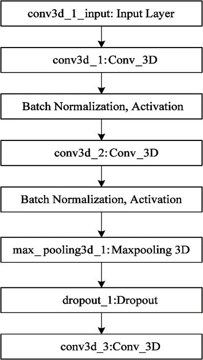
(a) The first structure

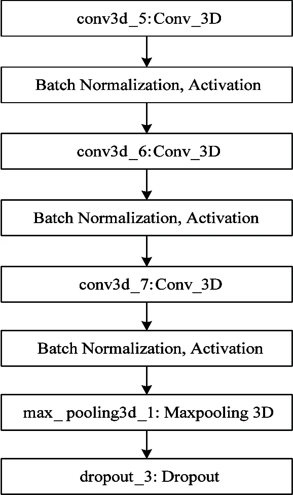
(b) The third structure

(c) Fully connected layer

1.4 Implementation of fusion network based on Keras framework

The fusion network is implemented on the basis of the pre-trained 3D-BN-VGG. A new ‘reshape’ layer and an LSTM unit layer are added, and the final output softmax layer is unchanged. The reshape layer separates the output eigenvectors of each video frame into a dimension, which serves as the time step length of LSTM. In order to improve the accuracy of classification, LSTM is used to process some sequence features which can not be extracted from 3D-BN-VGG. The network fusion structure is shown in Fig.3. The structure diagram of the newly added network layer is shown in Fig.4. The input of the ‘flatten_1’ layer is the output of 3D-BN-VGG. Through this layer, the output feature vector of each video frame is separated into one dimension, which is the time step length of the LSTM, and the data length of the LSTM input is 2 048, which is the length of the feature vector output from the convolutional network. The output feature length of the LSTM is 1 024. The feature vector of length 1 024 is sent to the ‘dense_1’ layer and they are classified by the softmax function. In order to avoid the loss of useful information in the downsampling of the pooling layer, the sampling window of the pooling layer in the pre-trained 3D-BN-VGG is changed from 2×2×2 to 2×2×1. In this way, the pooling layer will only sample in the 2-dimensional spatial domain, and the sequence features of the time domain can be completely preserved. Since the parameters of the convolutional layer have not changed, this does not affect the 3D-BN-VGG extraction time domain feature.

Fig.3 Fusion network

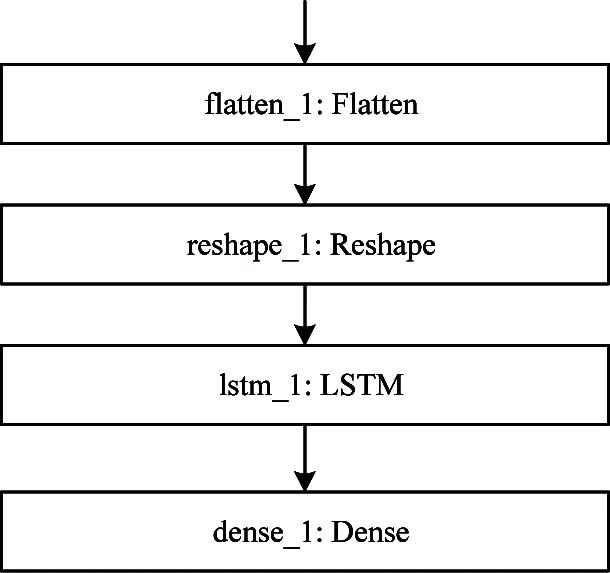
Fig.4 Keras framework structure of the fusion network

By describing each module of the network structure, the entire framework of the fusion network is obtained, as shown in Fig.5.

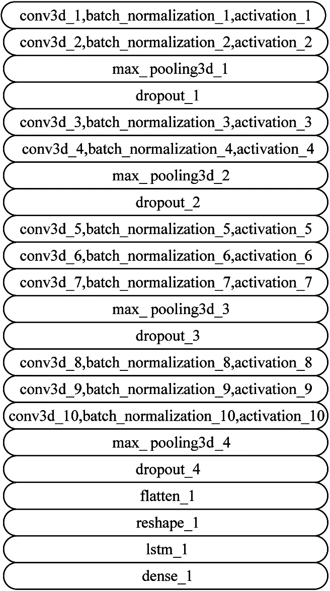
Fig.5 The structure of entire framework

2 Experimental results and analysis

2.1 Experimental hardware and software environment

The experimental environment used in the network training is shown in Table 1. In the experimental stage, the Keras framework is used to implement the specific network structure and conduct training and testing; Ubuntu is used as an experimental system; NVIDIA’s GeForce GTX1080Ti GPU is applied as a computing device in order to complete the computing tasks in the network training and testing phase. Since Keras’ back-end TensorFlow[18]has excellent data parallel acceleration for multiple graphics cards, the experimental phase uses two GTX1080Ti GPUs to speed up the training process. In addition, a large amount of training data needs to be read repeatedly in the training process, in order to speed up the training process, the training data is stored on the solid state hard disk.

Table 1 Experimental hardware and software environment

2.2 Data preprocessing

UCF-101 dataset is the largest public behavior recognition dataset at present. Video clips in the data set are collected from YouTube video website, which contains 101 categories of human behavior and 13 320 video clips. All the videos are collected from real life scenes, which is the most challenging behavior recognition data set at present. The average number of video clips in each class of UCF-101 dataset is about 130, and the length of the video clips is more than 5-10 s. Each video contains a complete process of human behavior, and the quality of data sets is good. At the same time, the resolution of all video clips is normalized to 320×240. The HMDB-51 data set includes 51 categories of human behavior and 6 849 video clips.Compared with UCF-101 data set, it contains fewer videos, and the length of each video clip is concentrated in 1-5 s, which has relatively less data. The overview of data sets is shown in Fig.6.

Both UCF-101 and HMDB-51 used are based on video sequence data. It is not feasible to directly use video sequences as input, so it is necessary to parse the video sequence into a picture format.

Since all video lengths are long and the average length is about 100 frames, it is not possible to put all of the selected video sequences into the network training. It adopts a video frame selection strategy of random starting frame: after selecting a video sequence as training data, the lengthNof the video frame is obtained by the number of images. Then it can use the random number generation function of the NumPy[19]to generate a random numberRin the range of 0 toN-32, and it uses the random number as the starting frame of the selected video frame, and theRtoR+31 frames of the video are selected as training data. It can generate more different training samples to achieve the purpose of data augmentation. For each video sequence, it can generateN-32 training samples, and since these samples start with different frames, the risk of over-fitting the same data multiple training is reduced. Experiments have shown that using this strategy increases the accuracy by 2%. The strategy for data processing in HMDB-51 is the same.

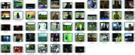
(b) HMDB-51

2.3 Fusion network training process

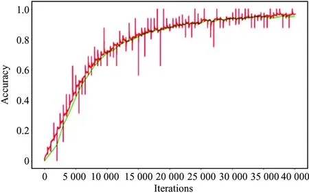
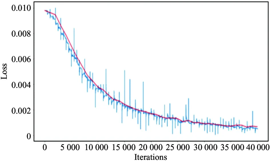
In the experimental stage, the UCF-101 data set is divided into 3 parts, of which 9 624 are used as training data, 1 896 are used as verification data, and 1 800 are used as test data. For the HMDB-51 data set, 4 794 are used as training data, 1 000 are used as verification data, and 1 055 are used as test data. The number of iterations of training is determined to be 40 000 times after multiple trials. Since the BN is used to accelerate the training, the initial learning rate is set to 0.1, the learning rate is 1e-6. In the training, the momentum is added to the SGD algorithm to update the parameters. When the network is trained, it is set to 0.9. The trained 3D-BN-VGG network parameters are used in the fusion network training to initialize the pre-network. It uses the transfer learning in the training process. Fig.7(a) is the accuracy curve and Fig.7(b) is the loss function curve.

(a) Accuracy curve

(b) Loss function curve

In Fig.7, When it only trains 3D-BN-VGG, the network is iterated by 130 000 iterations. In fact, the fusion network is iterated by 40 000 iterations during the training process. It can be seen that the fusion network which is trained using migration learning is faster, especially in the early stage of training, the accuracy has reached 60% by only 6 000 iterations.

2.4 Test indicators

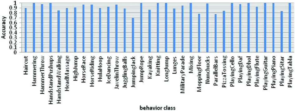
As shown in Fig.8, the test results are directly displayed for each class in the fusion network . The lowest accuracy of all kinds of tests is ‘WalkingWithGog’, with an accuracy of 69.79%.The accuracy of ‘ApplyLipstick’, ‘BlowingCandle’,‘Boxin-gSpeedBag’,‘CricketBowling’, ‘FrisbeeCatch’ and other classes is 100%, and the actions are relatively simple. According to the visual recognition results of each class, the reasons leading to the difference of each class are analyzed for further study. Although the complexity of each type of action, the similarity of action and background and many other reasons lead to the difference of recognition rate, there is little difference in accuracy between different classes. Table 2 and Table 3 give the overall data set accuracy, various average accuracy rates and various accuracy variances.

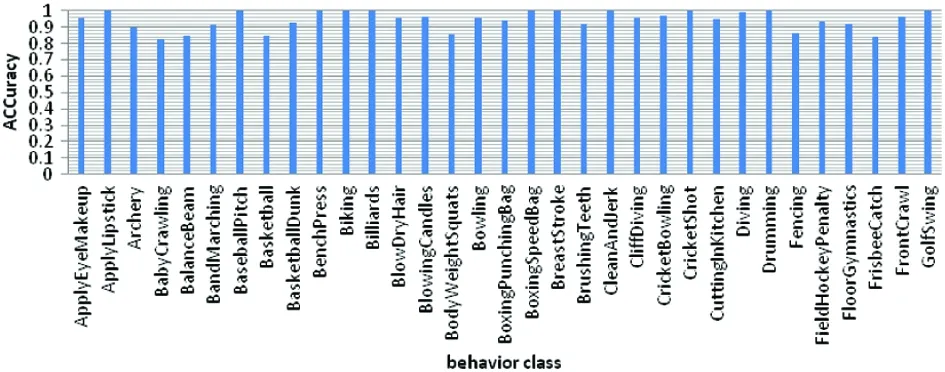
(a) The results in part I

(b) The results in part II

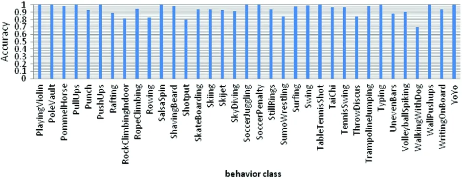
(c) The results in part III

Table 2 Accuracy statistics of 3D-BN-VGG

Table 3 Accuracy statistics of fusion networks

According to the statistical information of the fusion network accuracy, it can be found that the accuracy of the fusion network in each category is small, so the accuracy of the fusion network for different types of behavior recognition is relatively stable.

2.5 Choice of decision strategy

All tests are based on every 32 frames as an input data. For example, a sample video sequence containing 128 frames will have 4 input data and 4 classification results, and each classification result has independent statistical accuracy. The result of such statistics has a certain impact on the accuracy. For instance, if one of the 4 classification results is wrong, while the other 3 classification results are correct, the accuracy rate is only 75%. In order to avoid the inconsistency of multiple test results of the same sample, an improved decision-making strategy is proposed in the decision-making stage. The basic idea of the strategy is to fuse multiple test results of the same sample.

When the results are fused, the softmax output probabilities of the decision results of multiple input data of the same sample are fused, and then the consistent classification results are obtained. The experimental process directly averages the softmax output vectors of multiple input data of the same test sample, and the fusion method is as shown in Eq.(3).

(3)

Table 4 Comparison of accuracy before and after fusion using decision results

As can be seen from Table 4, the accuracy rates in the fusion network are increased by 0.5% on UCF-1 and by 0.77% on HMDB-51 after using the decision result fusion strategy.

2.6 Evaluation of test results

Table 5 shows the behavior recognition algorithm implemented. The test accuracy index on the specific data set is compared with the excellent research results in the field of behavior recognition at home and abroad. The experimental results prove the feasibility of the new idea of combining the 3D-CNN with LSTM to process the video sequence, and obtain better results. It is better than the best algorithms in Ref.[20] and Ref.[21]. At the same time, compared with the algorithm of two-dimensional CNN and LSTM network fusion realized in Ref.[17], the algorithm of 3D convolutional neural network and LSTM network realized has greatly improved the accuracy performance. It also shows that the algorithm of fusion network is a feasible and effective scheme in the field of human behavior recognition.

Table 5 Comparison of the accuracy of the algorithm and other excellent research results

Table 6 shows the comparison between the computational performance of the fusion network implemented and some other excellent research results. It can be found that the algorithm has a great advantage in speed.

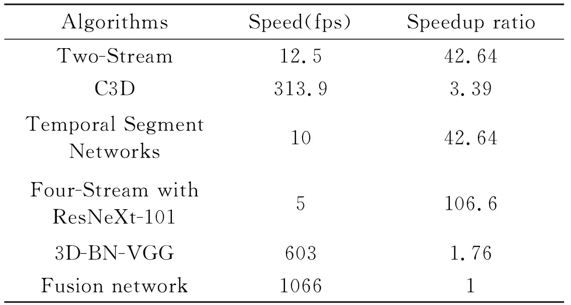
Table 6 Comparison of calculation speed between this algorithm and other excellent research results

2.7 Analysis of network parameters

There are 25 parameterized layers in 3D-BN-VGG with a total of 23 734 597 parameters, of which 23 722 437 are trainable parameters. Among the trainable parameters, the total connection layer parameters are 21 080 165, which account for 88.86% of the total parameters.The huge amount of parameters in the fully connected layer will greatly affect the generalization ability of the entire network. A higher Dropout discard rate is employed to reduce the risk of over-fitting of the fully connected layer.

Table 7 shows the amount of parameters for every layer of the fusion network. The parameter value of the whole fusion network is 15 324 485, which is nearly 2 times smaller than that of the 3D-BN-VGG network 23 734 597. The parameters of the convolutional layer are 2 633 952, accounting for 17% of all parameters. The parameters of the LSTM layer account for 82% of the total parameters quantity, and the last output layer’s parameters only account for 1%. The main reason for the decrease of the parameter quantity is that the full connection layer is removed.

Table 7 Parameters of each part of the fusion network

3 Contribution

Through the analysis of the previous sections, the contributions of this paper are as follows:

The choice of convolution core uses multiple small convolution cores stacking instead of large convolution cores, which deepens the depth of the neural network and reduces the parameters of the network.

The latest batch normalization algorithm is added to the network to improve the training speed.

Increasing Dropout layer reduces the risk of over-fitting.

Removing the full connection layer, which accounts for 88.86% of the total network parameters, and connecting the final output of the convolution layer directly to the reshape layer, the output eigenvectors of each video frame are separated into one dimension, LSTM network processes some sequence features that can not be extracted from 3D-CNN to improve the accuracy of classification. Through the analysis of Table 7, the amount of network parameters has also been reduced nearly twice.

Data preprocessing strategy reduces the risk of over-fitting of the same data after repeated training. Experiments show that using this strategy improves the accuracy by 2%.

After using decision fusion strategy, the accuracy of fusion network is improved by 0.5% on UCF-1 and 0.77% on HMDB-51.

Through the above improvements, compared with some excellent research results, the main contributions are as follows:

(1) The recognition rate is improved, as shown in Table 5.

(2) The calculation speed has been greatly improved, as shown in Table 6.

4 Conclusion

This work designs a fusion network combining 3D convolutional network and LSTM network. The algorithm is extended to 3D convolutional neural network.Compared with the fusion network of 2D convolutional neural network and LSTM, the advantages of the network implemented are: it can extract the front and rear frame information of video sequence in advance, which can improve the feature extraction ability of the algorithm. At the same time, in the network implementation, there is no need to use the batch size channel input from the network to replace the video sequence dimension, which is faster in the network implementation and training process. In the specific implementation, the fusion network does not use the full connection layer to reduce the output of the convolutional network. It avoids the loss of features, reduces the amount of parameters of the network and improves the generalization ability of the network. In the experimental stage, the performance of the fusion network implemented is verified on the specific data sets, and the accuracy is greatly improved compared with that of the 2D convolutional neural network.