Variational Inference Based Kernel Dynamic Bayesian Networks for Construction of Prediction Intervals for Industrial Time Series With Incomplete Input

Long Chen, Linqing Wang, Zhongyang Han, Member, IEEE, Jun Zhao, Senior Member, IEEE, and Wei Wang, Senior Member, IEEE

Abstract—Prediction intervals (PIs) for industrial time series can provide useful guidance for workers. Given that the failure of industrial sensors may cause the missing point in inputs, the existing kernel dynamic Bayesian networks (KDBN), serving as an effective method for PIs construction, suffer from high computational load using the stochastic algorithm for inference.This study proposes a variational inference method for the KDBN for the purpose of fast inference, which avoids the timeconsuming stochastic sampling. The proposed algorithm contains two stages. The first stage involves the inference of the missing inputs by using a local linearization based variational inference,and based on the computed posterior distributions over the missing inputs the second stage sees a Gaussian approximation for probability over the nodes in future time slices. To verify the effectiveness of the proposed method, a synthetic dataset and a practical dataset of generation flow of blast furnace gas (BFG) are employed with different ratios of missing inputs. The experimental results indicate that the proposed method can provide reliable PIs for the generation flow of BFG and it exhibits shorter computing time than the stochastic based one.

I. Introduction

IN industrial production process, e.g., iron and steel making process, there are lots of process variables which need to be monitored or predicted in order to guarantee the production reliability, safety and low economic cost [1]. Through the commonly implemented supervisory control and data acquisition (SCADA) system, industrial time series data of these process variables are collected, based on which one can build a prediction model [2], [3]. However, the high level noise and the missing data often corrupt the obtained industrial data,which makes it difficult for high prediction accuracy, while the workers on-site not only focus on the point estimate of the variables, but the reliability of the prediction as well [4].

As for the industrial time series prediction, lots of data-based methods are developed [5]–[7]. The most commonly used methods are those based on the artificial neural networks(ANNs) [8], the Gaussian processes [9], and the least square support vector machines (LSSVM) [10], etc. In [11], an effective noise estimation-based LSSVM model was reported to perform online prediction of the byproduct gas flow in steel industry. Besides, a Gaussian process based echo state networks(ESN) model was reported in [12] for prediction of the flow of coke oven gas and gasholder level in steel industry. However,these mentioned methods are all focused on the pointwise estimates, which failed to provide the reliability of prediction,and cannot deal with the situation of missing inputs.

A class of PIs based approaches can not only produce the predictive mean but also provide an interval with some confidence level, in which the bootstrap method, the Bayesian method, the mean-variance estimates (MVEs), and the delta method are usually combined with ANNs for such a task [13]–[15]. In addition, the PIs can also be constructed by using the fuzzy sets theory [16]. The delta method was first presented in[17], which was based on an assumption condition that the variance of all the samples was identical. However, such an assumption was rather difficult to be satisfied when facing with real world problems. The Bayesian theory-based PIs construction usually relied on the prior distribution of the samples, especially when the sample amount was relatively small [18]. The MVE method assumed that the network could accurately estimate the target with the least computational load[19]. However, due to the uncertainties in practice, the generalization capability of the NN is insufficient. Besides, in[20], an ensemble model containing a number of reservoir computing networks was employed by using the bootstrap techniques, which was applied to the prediction of practical industrial data. However, the aforementioned methodologies are only formulated for the complete inputs, and when encountering the incomplete inputs one has to perform a data imputation procedure for the missing inputs before prediction.

Fig.3. KDBN structure for noisy Mackey-Glass time series prediction.

III. Experiments

To verify the effectiveness of the proposed inference method for the KDBN (KDBN-VI), a synthetic dataset and a practical industrial dataset are considered here.

A. A Synthetic Dataset

In this section, we employ the synthetic Mackey-Glass data.The Mackey-Glass equation is a differential equation with time delay, as formulated by

Here, the parameters a, b, and τ in (19) are set to be 0.2, 0.1,and 17, respectively. A time series of Mackey-Glass is generated from (19) by a numerical method. The length of this sequence is 600. For the purpose of verifying the performance of the proposed method when facing with the noisy data, we add a Gaussian white noise with the variance 0.001 into this generated time series.

In this experiment, th(e kernel fun)ction is Gaussian kernel function, K(x,xi)=exp||x−xi||/2b2. The 8-fold cross validation is used to determine the optimal value of b and the order of the KDBN. Finally, the order of the trained KDBN is set to be 30, and the kernel parameter b is set to be 1.673. Fig.3 shows the trained KDBN for the noisy Mackey-Glass data,where the parameters of the nodes after the 31st time slices share those of the 31st node. Besides, the experimental environment is the WindowsTMoperating system configured on a 3.4 GHz Intel Core i7-3770 chipset and 4 GB of RAM.The programming was completed in MATLABTM2014.

To quantify the performance of the construction of PIs, two indicators including the root mean square error (RMSE) and the coverage width-based criterion (CWC) are adopted here.

where n is the number of predicted points, Yiis the observed value and Fiis the predicted mean value. The RMSE aims to indicate the mean errors of the prediction. Besides, as for the interval performance, one can employ the CWC [7], which is a kind of combined index based on the PI coverage probability(PICP) and the mean PI width (MPIW).

and

where η and µ are two hyper-parameters, R denotes the range of the data, and ciequals 1 when the corresponding target is covered by the predicted coverage; otherwise, it equals 0. Uiand Liare, respectively, the upper and the lower bounds. PICP is measured by counting the number of target values covered by the constructed PIs. And NMPIW is the normalized MPIW showing the average width of PIs. The smaller it is, the better the performance, and the smaller the PICP is, the better the performance of PIs is.

To verify the performance of the proposed method, this study compares the experimental results of several other methods of PIs construction, including the KDBN with weighted likelihood inference (KDBN-WL) [25], the Bayesian multiple layer perceptron (Bayesian MLP) [13], and the bootstrap-based echo state networks (Bootstrap ESN) [20].The Bayesian MLP and the bootstrap ESN are the NNs based PIs construction methods. In the KDBN-WL, the number of samples in the WL algorithm is set to be 500. In the Bayesian MLP, the number of hidden nodes is set to be 30, and in the Bootstrap ESN, the number of the ESNs is 20. In these experiments, the hyper-parameters defined in (21) are set to be 10 and 0.95, respectively. The nearest neighbor imputation method is firstly conducted for imputing the incomplete inputs before performing inference with the Bayesian MLP and the Bootstrap ESN. Table I lists the statistical results of these aforementioned methods for the noisy Mackey-Glass data with different missing input ratios (20 independent experiments are performed). This table shows that the PIs performances (CWC, PICP, and NMPIW) of the KDBN-VI and the KDBN-WL are very similar, but the inference time of the KDBN-VI is much smaller than that of the KDBN-WL.Besides, the KDBN based methods produce better prediction performance than the other two NNs based methods.

TABLE I Comparison of the Prediction Results for Different Methods Under Different Missing Percentage of Inputs for the Noisy Mackey-Glass Data

Fig.4. Illustration of the generation of BFG.

Fig.5. Illustration of missing points. (a) A segment of the generation flow of BFG with missing points; (b) An example of missing points in an input vector [25].

B. A Practical Industrial Dataset

In steel industry, the BFG produced by blast furnace, can serve as the secondary energy. Therefore, it is significant to schedule the BFG which is generated from blast furnaces, and part of it is consumed by a number of hot-blast stoves before transporting into the pipeline network, as illustrated in Fig.4.These hot-blast stoves are often switched on or off, which makes large fluctuation of the BFG flow and the instability of the pressure of the gas in the pipeline network. Thereby, it is important to predict the generation flow of the BFG for the energy scheduling.

Fig.6. A KDBN for the flow of the BFG.

Through the SCADA system, the BFG data will be obtained in real-time, however, complex industrial environment may cause the failure of the sensors, which will lead to missing points in the input vector for a trained prediction model.Fig.5(a) presents a time series of the generation flow of BFG with missing points, where the locations marked by circles denote the missing points, and Fig.5(b) illustrates an example of missing points in input vector, where the circles in the solid line box denote the input vector of the model, and the hollow ones denote the value-missed variables in input vector.

A period of the generation flow of BFG, coming from the SGADA system of a steel plant in China in July 2016, serves as the experimental data in this study. The sampling period of these data is one minute. This study conducts the experiments under different missing ratios of inputs. The number of the sequences in the training set is 500, of which the length of each sequence is 80. The kernel function is the Gaussian kernel function. The order of the trained KDBN is set to be 45, and the kernel parameter b is set to be 834.45 by using the 10-fold cross validation. Fig.6 shows the trained KDBN for the generation flow of the BFG, where the parameters of the nodes after the 46th time slice share the 45th node.

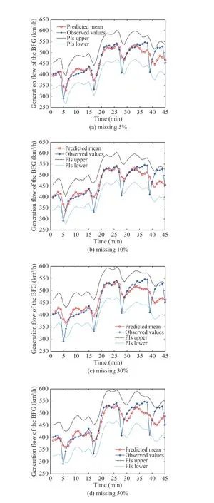
Fig.7 presents the experimental results of the proposed KDBN-VI with different missing input ratios including 5%,10%, 30%, and 50%, where 95% confidence level are shown.As shown in Fig.7, with the increase of the missing ratios, the KDBN-VI can exhibit a decline in the prediction quality,while even when the missing ratio of input is very large (e.g.,50%) the proposed KDBN-VI still shows a good performance for PIs construction. This means that the KDBN-VI has a high stability for the flow of the BFG with different levels of missing proportions. Besides, the inference time of this method is generally less than one second, which is very fast in the perspective of the industrial demands of real time prediction.

Similarly, to further verify the performance of the proposed method for the BFG data, this study compares the experimental results of several other methods of PIs construction, including the KDBN-WL [25], the Bayesian MLP [13], and the bootstrap ESN [20]. Table II lists the statistical results of these aforementioned methods for the generation flow of the BFG (50 independent experiments are performed). From this table, one can see that the KDBN based methods (the KDBN-VI and the KDBN-WL) exhibit relatively lower prediction error than the other two methods(the Bayesian MLP and the bootstrap ESN), refer to the values of the indicator RMSE. The prediction performances of the KDBN-VI and the KDBN-WL are similar, while the proposed KDBN-VI is much faster than the KDBN-WL. That is, the proposed one is more suitable for the industrial demand on real time inference than the KDBN-WL.

Fig.7. Experimental results of the KDBN-VI for the generation flow of the BFG with different missing ratios: (a) missing 5%; (b) missing 10%; (c)missing 30%; (d) missing 50%.

TABLE II Comparison of the Prediction Results for Different Methods under Different Missing Percentage of Inputs for the BFG Data

IV. Conclusions

This study addresses the problem of inference of the kernelbased DBN by using a variational inference based method with two stages. The first stage involves the computation of the analytical posterior distributions over the nodes of missing values approximately by using a local linearization based variational inference, and the second stage makes a Gaussian approximation for the posteriors over the predictive nodes in the future time slices. The proposed inference method avoids the time-consuming stochastic sampling scheme as employed in the original WL algorithm. The experimental results indicate that the proposed method is much faster than the WL algorithm, and it can produce reliable PIs for industrial demands.

This study only considers the input uncertainty in the conditional mean value (see (1)). Therefore, the future work will aim to tackle the inference problem with the input uncertainty both in the mean and variance by using variational inference, which is more complex since the approximation cannot be done by the first order Taylor expansion when considering the input uncertainty in variance.

Appendix Computations of Expectations In Variational Inference

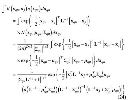
The details of the computation of expectations in (12) and(13) are given as follows. The missing input vector exists in the kernel function of the nonlinear mean function. Therefore,these expectations involve the integration of the kernel and the posterior over the missing input vector xqu. Assume that the variational posterior distributions over xquare expressed as a Gaussian form, i.e., q(xqu)=N(xqu|µqu,Σqu) with mean vector µquand covariance matrix Σqu, the integration is given by

where K(xqu,xj) is the kernel function of the xqu, and L denotes the diagonal length scale parameters.