Arbitrary-Order Fractance Approximation Circuits With High Order-Stability Characteristic and Wider Approximation Frequency Bandwidth

Qiu-Yan He, Yi-Fei Pu, Bo Yu, and Xiao Yuan

Abstract—This paper discusses a novel rational approximation algorithm of arbitrary-order fractances, which has high orderstability characteristic and wider approximation frequency bandwidth. The fractor has been exploited extensively in various scientific domains. The well-known shortcoming of the existing fractance approximation circuits, such as the oscillation phenomena, is still in great need of special research attention.Motivated by this need, a novel algorithm with high orderstability characteristic and wider approximation frequency bandwidth is introduced. In order to better understand the iterating process, the approximation principle of this algorithm is investigated at first. Next, features of the iterating function and frequency-domain characteristics of the impedance function calculated by this algorithm are researched, respectively.Furthermore, approximation performance comparisons have been made between the corresponding circuit and other types of fractance approximation circuits. Finally, a fractance approximation circuit with the impedance function of negative 2/3-order is designed. The high order-stability characteristic and wider approximation frequency bandwidth are fundamental important advantages, which make our proposed algorithm competitive in practical applications.

I. Introduction

STUDIES show that the fractional calculus is now the most appropriate description for most phenomena and their intrinsic essence in nature, such as diffusion processes [1]–[3],electrolytic chemical analyses [4], [5], and biological systems[6], [7]. Owing to the properties of long-term memory, nonlocality, and weak singularity, the fractional calculus has been widely used in various scientific fields, such as nonlinear control systems [8]–[20], fractional-order chaos systems[21]–[24], neural networks [25]–[30], and fractional-order circuits and systems [31]–[34].

As the physical realization of fractional calculus, the fractor is a burgeoning new circuit element with characteristics of the fractance which is a portmanteau of the fractional-order impedance. The ideal fractor does not currently exist and its approximate physical realization is called a fractance approximation circuit (FAC) [35].

FACs can be classified into two types. The first type is constructed directly or by modeling some phenomena of electrochemistry or other scientific fields, such as the 2h-type fractal tree FAC [35], the scaling fractal-lattice FAC [36],[37], the fractal-ladder FAC [38], , and fractal-chuan FAC[38]–[40]. The second is to design a rational function approximating to the irrational impedance function of the ideal fractor, then a circuit is synthesized to provide the corresponding rational function, such as the Oustaloup algorithm [41], the Carlson’s iterating rational approximation algorithm [42]–[44], etc. There are also some single type fractors [45], [46].

There exist the operational oscillation phenomena in the frequency-domain characteristics of the above mentioned approximate realizations of the fractor except the Carlson’s iterating rational approximation algorithm. The Carlson’s iterating rational approximation algorithm, proposed by Carlson and Halijak, is that the rational approximation of the fractance of −1/n-order has been transformed into the iterating solution of the root of an n-th two-term equation [42]. The predistortion exponent δ=0 has been introduced to speed up the convergence of this iterating process [42]. In view of the high order-stability characteristic, the Carlson’s iterating rational approximation algorithm has been generalized to approximate to arbitrary-order fractances in [35], [43], [44].Whether this kind of generalization is possible and what characteristics the impedance function Zk(s) should possess,have been explored in [43]. Characteristics of the generalized iterating function and approximation performance of this generalized iterating algorithm have been discussed and analyzed in detail in [44]. Both papers concentrate on the situation where the predistortion exponent δ equals zero. An algorithm with the value of the predistortion exponent in the range −1 ≤δ ≤1, is investigated in this paper, including the design of the corresponding FACs. Compared to other that is

Whether the impedance function sequence {Zk(s)} possesses fractional-order operation characteristics of the ideal fractor and can be realized with existing electronic elements, it still needs to satisfy these basic properties: computational rationality, positive reality principle, and operational validity[35], [43], [44]. Computational rationality means that there only exist rational computations in Zk(s) and ensures that the impedance function is a rational function. From (13), we know that the impedance function calculated through the iterating formula satisfies computational rationality when choosing the rational initial impedance Z0(s). Positive reality principle requires zeros and poles of the impedance function placed in the left half plane or on the imaginary axis of splane, then the impedance function can be realized with a causal and stable network. The operational validity signifies that the impedance function takes on operational characteristics of the ideal fractor.

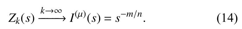
Along with the amplitude-frequency and phase-frequency characteristics; the order-frequency and F-frequency characteristics introduced in [35], [47], all are used to represent frequency-domain characteristics of the impedance function Zk(s). For a fractional-order system, the operational order is a key issue. It is necessary to introduce the order-frequency characteristic to represent the operational order. The F-frequency characteristic denotes the lumped characteristics quantity of FACs and plays an important role in designing FACs.Therefore, the Laplace variable s is substituted with the Fourier frequency variable Ω or the frequency exponent variable ϖ, namely.

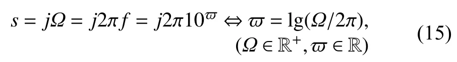
then the frequency-domain characteristics of the ideal fractance I(µ)(j2π10ϖ) include

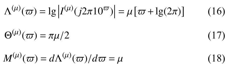
where Λ(µ)(ϖ), Θ(µ)(ϖ), and M(µ)(ϖ) are the amplitudefrequency, phase-frequency, and order-frequency characteristics of the ideal fractor, respectively.

In the same way, the frequency-domain characteristics of the impedance function Zk(j2π10ϖ) can be represented as follows:

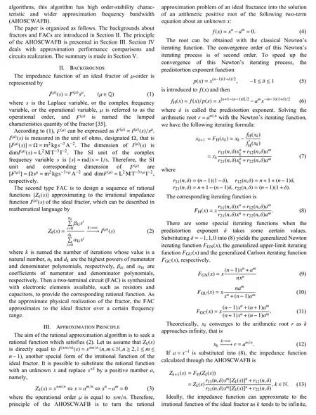
where Λk(ϖ), Θk(ϖ), and Mk(ϖ) are the amplitudefrequency, phase-frequency, and order-frequency characteristics of the impedance function, respectively. The F-frequency characteristic of the impedance function is defined as

According to the frequency-domain characteristics of the impedance function Zk(j2π10ϖ), the operational validity falls into three parts.

1) Validity of the amplitude-frequency characteristic

2) Validity of the phase-frequency characteristic

3) Validity of the order-frequency characteristic

If the impedance function Zk(j2π10ϖ) can approximate to the irrational function of the ideal fractor, the frequencydomain characteristics of the impedance function satisfy(23)–(25) automatically.

For the value of the operational order in the range 0<µ<1,the impedance function can be obtained by substituting a=s into (8) or making directly reciprocal transformation to (13).Therefore, the AHOSCWAFB can realize the rational approximation of fractances with values of the operational order in the range of −1<µ<0 and 0<µ<1.

IV. Experiment and Analysis

A. Features of the Iterating Function

Plots of the iterating function FH(x) for different predistortion exponents are shown in Fig.1. All these iterating function curves take on uniqueness of the positive root and local convergence. The two properties state that these iterating processes can converge to the arithmetic root r as k approaches infinity. It is also noted that only when the predistortion exponent δ is equal to zero, does the iterating function FGC(x) possess strictly global regularity.

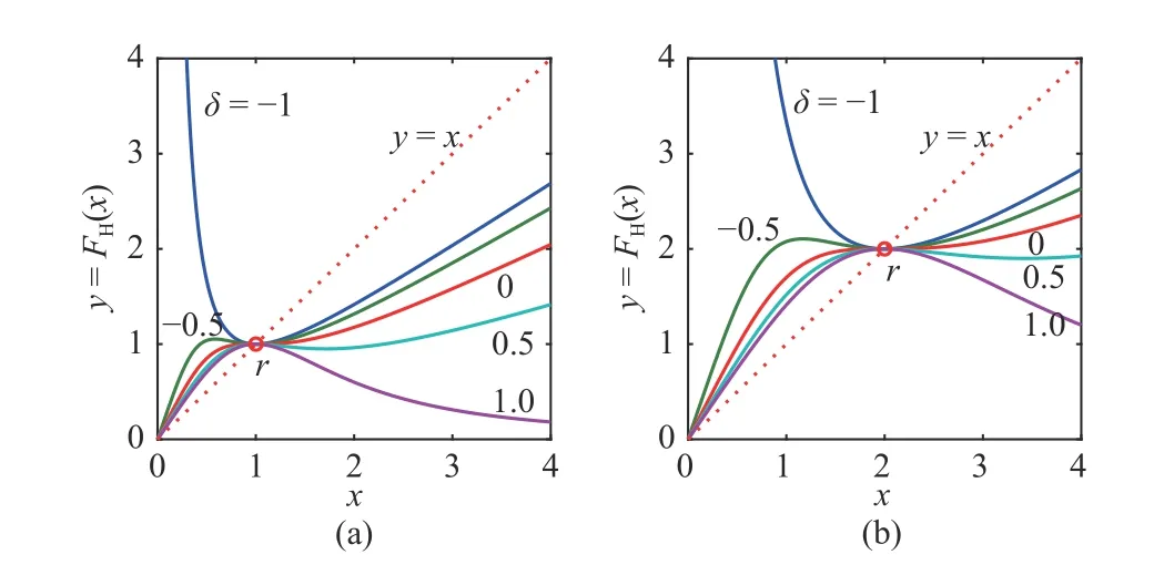
Fig.1. Plots of the iterating function for different predistortion exponents,n =3 and m=2: (a) a=1; (b) a=2n/m.

For a given operational order µ and a certain predistortion exponent δ, these plots of the iterating function FH(x) for different positive real numbers a, shown in Fig.2(a), are selfsimilar. Such property is specially obvious in the double logarithmic coordinate (Fig.2(b)). Therefore, it is necessary to make normalization processing and double logarithmic transformation to the iterating function FH(x).

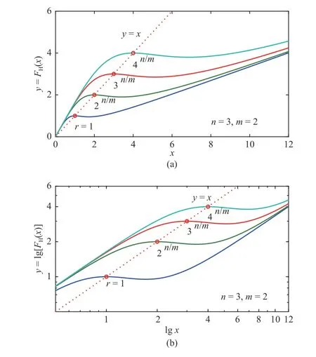
Fig.2. Plots of iterating functions with different positive real numbers a and δ=0.5: (a) double linear coordinate; (b) double logarithmic coordinate.

Let

where α is referred to as the normalized exponent variable.Making normalization processing and taking logarithmic operation on both sides of (8) produce

Considering r=am/n⇔am=rn, the normalized exponential form of FH(x) can be simplified as

The left asymptote function of the normalized exponential function is expressed as follows:

Likewise, the right asymptote function of the normalized exponential function is represented as

Plots of the normalized exponential functions with different predistortion exponents δ are represented pictorially in Fig.3.It is apparent that the plot of the normalized exponential function with δ can be obtained through the plot of the normalized exponential function with −δ rotated 180 degrees.

B. Frequency-Domain Characteristics of the Impedance Function

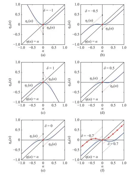
Fig.3. Plots of normalized exponential functions with different predistortion exponents δ and n=3: (a) δ=−1; (b) δ=−0.5; (c) δ=1; (d)δ=0.5; (e) δ=0; (f) δ=±0.7.

For the AHOSCWAFB, it is already known that this initial impedance function should be a rational function according to the computational rationality. The selection of initial impedances for every operational order is tested by experiments. Some frequently encountered examples are included in Table I.

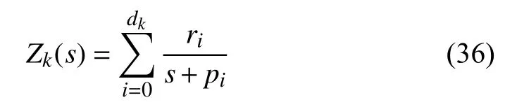
1) High Order-Stability Characteristic: Taking µ=−1/3,−3/4,−5/6 as examples with Z0(s)=R,1/s,1/s, respectively,the impedance functions can be obtained by (13). The corresponding frequency-domain characteristics are displayed in Fig.4, seeing the solid lines. The dotted lines typify the frequency-domain characteristics of the corresponding ideal fractor. The frequency-domain characteristics of these calculated impedance functions overlap with those of the corresponding ideal fractors in a certain frequency range. The calculated impedance functions take on operational characteristics of the ideal fractor in a certain frequency range and then the operational validity is satisfied. Since the initial impedance functions used are rational, the impedance functions possess the computational rationality. Because all zeros and poles of the impedance functions are placed in the left half plane or at the origin of s-plane, the positive reality principle is satisfied and then circuit networks can be synthesized according to the impedance functions. The impedance functions satisfy the three basic properties. In addition, there exist no oscillation phenomena in the valid

frequency range. The impedance function calculated by the algorithm is with high order-stability characteristic.

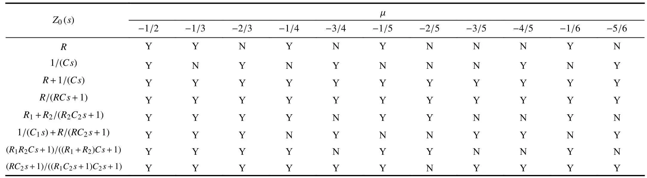
TABLE I Selection of Initial Impedances for Different Operational Orders

In order to show the degree of approximation of the impedance function calculated by the AHOSCWAFB to the irrational function of the ideal fractor, the relative error functions are introduced to make approximation error analysis, as defined below:

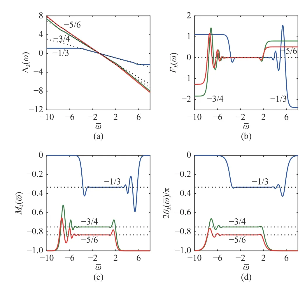
Fig.4. Frequency-domain characteristics for different operational orders with k=5 and δ=0.5: (a) amplitude-frequency characteristic; (b) F-frequency characteristic; (c) order-frequency characteristic; (d) phase-frequency characteristic.

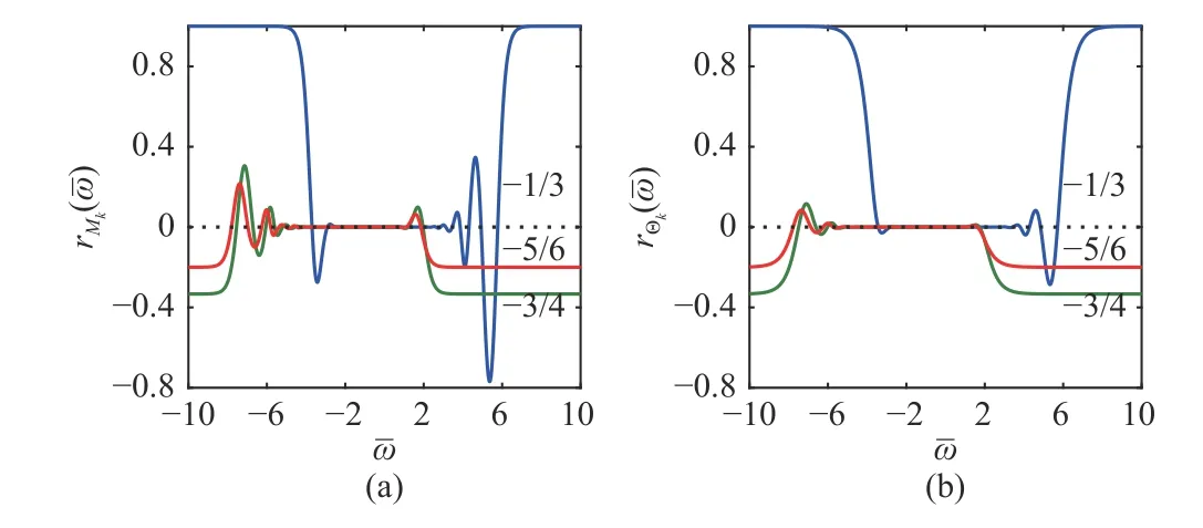
Fig.5. Relative errors of frequency-domain characteristics for different operational orders with k=5 and δ=0.5: (a) order-frequency characteristic;( b) phase-frequency characteristic.

In addition, a brief analysis is made of the high orderstability characteristic of the AHOSCWAFB. We know the impedance function can be expressed in the form of zeros and poles, that is

where r,l, and c denote a resistance, an inductance, and a capacitance, respectively. ziand pirepresents the ith zero and pole of the impedance function, respectively. A certain impedance function may vary and some items may be omitted.Generally, zeros and poles are negative real numbers or in the original point for most of FACs. While for the impedance function calculated by the AHOSCWAFB, there exist conjugate zeros and poles.

A system with the impedance function can be divided into a series of subsystems based on (33). Taking µ=−m/n=−2/3 with the initial impedance Z0(s)=1/s as an example, the frequency-domain characteristics of each subsystem and the entire system are shown in Fig.6. The bold black curve represents the frequency-domain characteristics of the entire system and the others represent those of each subsystem. The oscillation amplitude of the AHOSCWAFB is equal to 0,which shows the AHOSCWAFB is with the high orderstability characteristic.

2) Wider Approximation Frequency Bandwidth:Approximation frequency bandwidth B of an impedance function Zk(s) increases with the increase of value of k, as

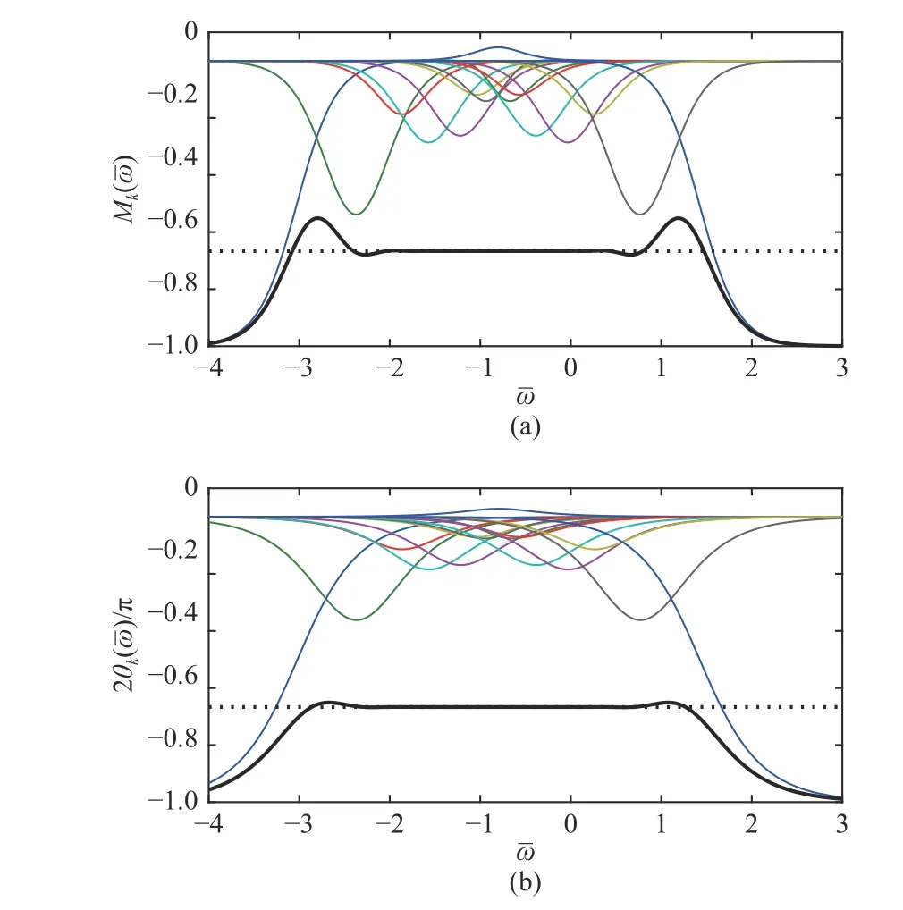
Fig.6. Frequency-domain characteristics of the entire system and each subsystem with µ=−2/3 and k=3: (a) order-frequency characteristic; (b)p hase-frequency characteristic.

Fig.7. Frequency-domain characteristics for different values of k withµ=−2/3 and Z0(s)=1/s: (a) order-frequency characteristic; (b) phasef requency characteristic.

shown in Fig.7. Ideally, as k tends to infinity, the impedance function Zk(s) can converge to the irrational function of fractor I(µ)(s) in the entire frequency range.

The valid approximation frequency bandwidth B of an impedance function approximating to that of the ideal fractor is approximately equal to

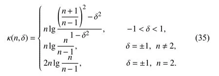
where κ(n,δ) is the approaching rate which describes how the valid approximation frequency bandwidth changes over the number of iterations k and can be expressed as

The approaching rate is determined by both the predistortion exponent and n. For the same value of n, even for different operational orders, approaching rates are identical according to (35). The approaching rate tends towards 4lge as n approaches infinity. Therefore, considering different operational orders and the value of the predistortion exponent in the range |δ|<1, the approaching rates are portrayed in Fig.8.As can be seen from this figure, when the predistortion exponent is equal to zero, the approaching rate is the smallest for every operational order. The value of the approaching rate increases as the absolute value of the predistortion exponent is increased. When the operational order and the value of k are chosen, the approximation frequency bandwidth increases with the increase of the absolute value of the predistortion exponent. When the predistortion exponent is equal to zero,the approximation frequency bandwidth is the smallest. This conclusion also explains why the impedance function calculated by the AHOSCWAFB is with wider approximation frequency bandwidth.

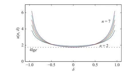
Fig.8. Approaching rates for different operational orders.

With the operational order µ=−m/n=−2/3 as an example,the frequency-domain characteristics of impedance functions for different predistortion exponents are depicted in Fig.9,seeing the solid lines. The dotted lines typify the frequencydomain characteristics of the ideal fractor s−2/3. Although there exist operational oscillation phenomena out of band when the predistortion exponent δ is not equal to 0, the approximation frequency bandwidths are wider, compared with the case of δ=0. According to the aforementioned discussion, we have already known that the iterating function FH(x) is not globally regular when the predistortion exponent δ is not equal to zero. The non-global regularity is the main

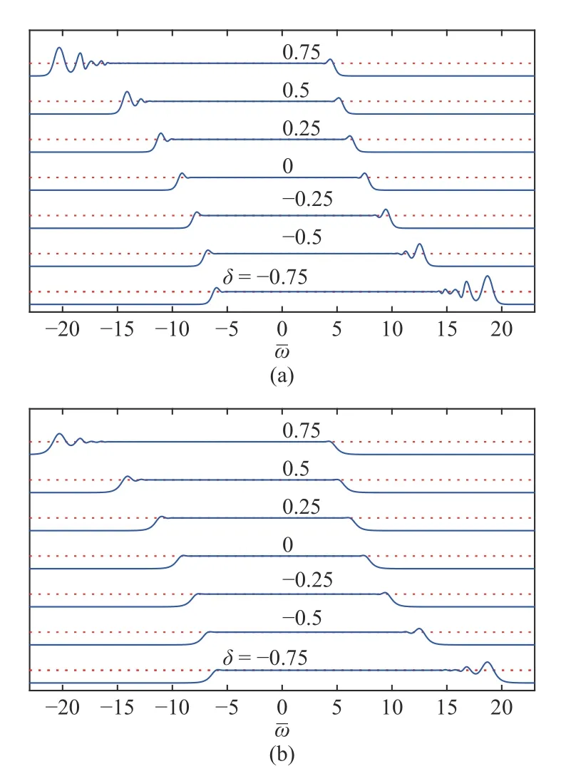
Fig.9. Frequency-domain characteristics for different predistortion exponents with µ=−2/3, k=10, and Z0(s)=1/s: (a) order-frequency characteristic; (b) phase-frequency characteristic.

reason why there exist operational oscillation phenomena out of band in frequency-domain characteristics.

Approaching rates of impedance functions with different predistortion exponents are included in Table II. Subscripts O and P correspond to the order- and phase-frequency characteristics, respectively. It is really that the approximation frequency bandwidth increases with the increase of the absolute value of the predistortion exponent.

Considering two different predistortion exponents δ=0.4 and δ=0.8, approaching rates of impedance functions with different operational orders are listed in Tables III and IV,respectively.

As can be seen from these tables, approaching rates are the same as the theoretical values according to (35). Given a predistortion exponent, approaching rates are identical for the same value of n, even for different operational orders. As we have discussed, the plot of the normalized exponential function with δ can be obtained through the plot of the normalized exponential function with −δ rotated 180 degrees.Therefore, the approaching rate with the predistortion exponent δ is equal to the approaching rate with the opposite of this predistortion exponent, namely, κ(n,δ)=κ(n,−δ). For the same operational order and values of the predistortion exponent δ in the range 0<|δ|<1, the approaching rate is greater than κ(n,0) and is getting larger and larger with the increase of the predistortion exponent. That is to say, the greater the absolute value of the predistortion exponent δ whose value in the range 0<|δ|<1, the wider the approximation frequency bandwidth.

C. Performance Comparison

Comparisons about approximation performance between the AHOSCWAFB and other types of FACs are made in this section.

The scaling fractal-ladder FACs (SFLFACs) and the scaling fractal-chuan FACs (SFCFACs) can achieve the rationalapproximation of fractances of arbitrary order and the corresponding optimized circuits have been discussed in ,[40]. Another optimization method of SFCFACs has been proposed by Adhikary in [39]. The corresponding circuit is denoted by SFCFACs_A. The classical negative-half-order lattice-type FAC, denoted by LATTICE, also can realize the rational approximation of fractances of arbitrary order after making scaling extension [36], [37]. The Oustaloup algorithm,a matching algorithm of recursive distribution of zeros and poles, also can realize the rational approximation of fractances of arbitrary-order [41], [48], [49].

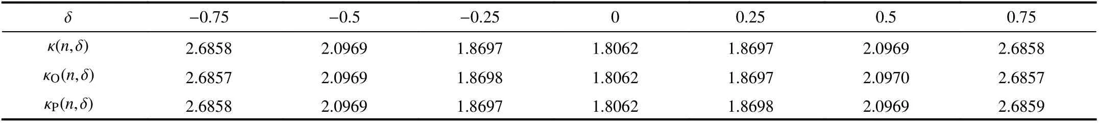
TABLE II Approaching Rates of Impedance Functions With µ=−2/3, Z0(s)=1/s and Different Predistortion Exponents

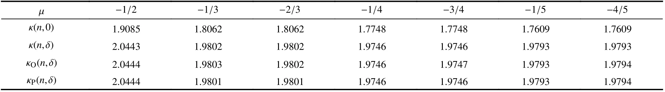
TABLE III Approaching Rates of Impedance Functions With δ=0.4 and Different Operational Orders

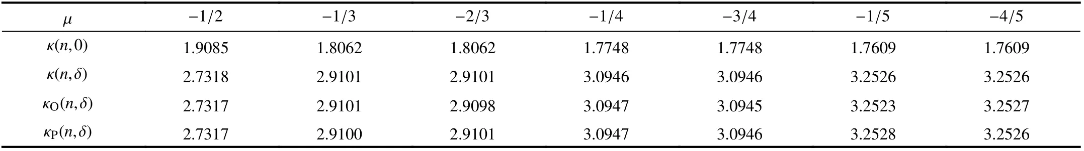
TABLE IV Approaching Rates of Impedance Functions With δ=0.8 and Different Operational Orders

Considering the roughly same approximation frequency bandwidth, the frequency-domain characteristics for different FACs are depicted in Fig.10. Results of comparisons of approximation performance are summarized in Table V. In the valid approximation frequency range, the oscillation amplitudes of the frequency-domain characteristics obtained by other FACs are not equal to zero and there exist operational oscillation phenomena in band, whereas the frequency-domain characteristics of the impedance function calculated by the AHOSCWAFB are smooth and consistent with those of the irrational function of the ideal fractor and the oscillation amplitude is equal to zero. In addition, the Ffrequency characteristic is a fixed value in the valid approximation frequency range, which makes the AHOSCWAFB more suitable for applications with high-order stability.

The highest power of the impedance function means the complexity of a circuit. The highest power of the impedance function Z3(s) acquired by the AHOSCWAFB is 22, while that of the impedance function obtained by the Oustaloup algorithm equals 9. The stages of SFLFACs, SFCFACs,SFCFACs_A, and LATTICE are equal to 7, 7, 6, and 6,respectively. Therefore, the complexity of circuit designed by the AHOSCWAFB is larger, compared with other FACs.

For other FACs, oscillation phenomena of frequencydomain characteristics are inherent properties. Although the oscillation amplitude can be reduced by adjusting circuit parameters, the oscillation phenomena do not disappear and the circuit stage is increased. Despite the complexity of circuit is comparatively high, the excellent approximation performance shows that the AHOSCWAFB is also a good direction of the research.

D. Implementation of Circuit

In this section, the aim is to design the FAC to provide the impedance function obtained through the AHOSCWAFB.This kind of circuit is called the FAC with high order-stabilitycharacteristic and wider approximation frequency bandwidth(FACHOSCWAFB).

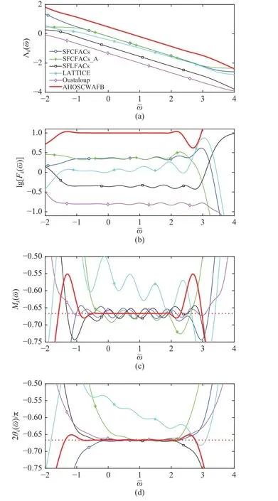
Fig.10. Approximation performance comparisons with the scaling factor equal to 1/5 for other FACs and the Oustaloup algorithm: (a) amplitudefrequency characteristic; (b) F-frequency characteristic; (c) order-frequency c haracteristic; (d) phase-frequency characteristic.

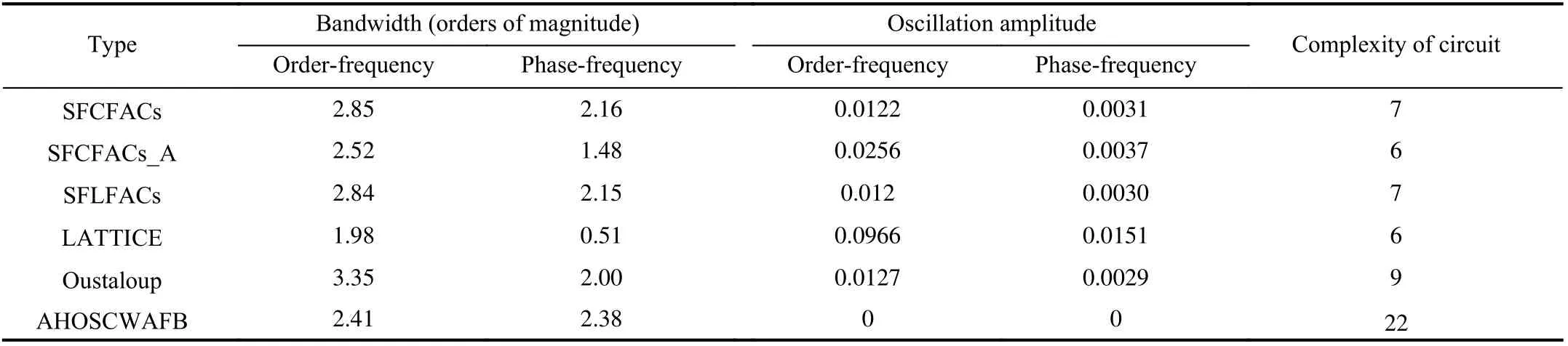
TABLE V Approximation Performance Comparison

Given a certain operational order µ=−m/n and choosing an appropriate initial impedance function, the impedance function can be calculated using (13). By using the partial fraction expansion, the impedance function can be rewritten in the following form:

where pidenotes the pole of the impedance function and rirepresents the residue of the corresponding pole. Therefore,the impedance function can be realized with commercially available circuit elements.

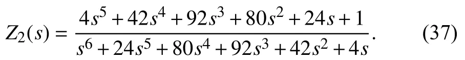
Take the operational order µ=−2/3 with the predistortion exponent δ=0 and Z0(s)=1/s as an example. According to(13), the impedance function Zk(s) after iterating 2 times is

Partial fraction expansion applied to (37) leads to the following relationship:

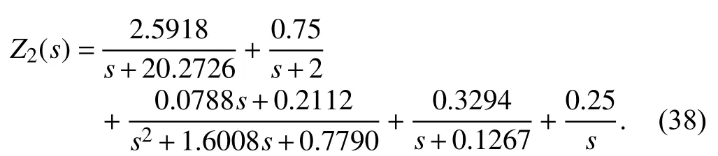
For the first term on the right-hand side of (38), it can be realized with the 1/2.5918-F capacitor in parallel with the 2.5918/20.2726- Ω resistor. The second and fourth terms can be achieved in the same way. The third term can be obtained with a capacitor, a resistor and a series combination of an inductor and a resistor in parallel. The last term is a capacitor.All these terms are in series.

If we use the calculation results in (38) as values of the used circuit elements directly, the approximation frequency is too small to measure. It is possible to measure circuit characteristics with resistance of each resistor magnified 105times and capacitance of each capacitor reduced 10−10times. Such modifications shift the approximation frequency to high frequency with five orders of magnitude. However, the modifications make the lumped characteristics quantity too large and the current flowing through the circuit too weak to measure. A viable solution for this problem is that the impedance function is multiplied by a coefficient 1/70 without changing the order-frequency and phase-frequency characteristics. Such alterations make the amplitude of this impedance function be decreased 70 times. Therefore, the ultimate circuit parameters are displayed in Fig.11.

The negative resistor in the FACHOSCWAFB is realized by the negative impedance converter shown in Fig.12.

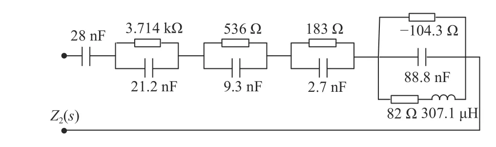
Fig.11. FACHOSCWAFB with µ=−2/3.

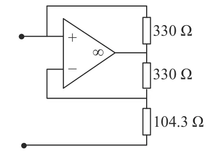
Fig.12. Negative impedance converter.

These elements in Fig.11 can be realized with resistors,capacitors, and active elements. All these circuit elements can be purchased at the market. The type of the operational amplifier used above is OP37. The practical testing system is represented in Fig.13. The types of the signal generator, the oscilloscope, the current probe, and the current amplifier used in this experiment are NDY EE16330, Tektronix TDS 1012CEDU, TCP312A, and TCPA300, respectively.

Fig.13. Testing system.

Amplitude and phase spectra of the above FACHOSCWAFB through simulation by the Multisim are pictured in Fig.14 and in accordance with those of the modified impedance function simulated by the MATLAB. As can be seen from this figure, the modified impedance function can approximate to the fractance of −2/3-order and the FACHOSCWAFB can be viewed as the approximate realization of the ideal fractor of −2/3-order in a certain frequency range.

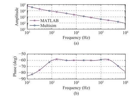
Fig.14. Frequency spectrums of the FACHOSCWAFB: (a) amplitude spectrum; (b) phase spectrum.

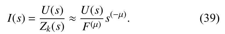
The input voltage U(s) and current I(s) are referred to as the Laplace transformations of time-domain voltage and current signals, respectively. Therefore, the relationship between the input voltage and current can be represented as follows:

The input current can be viewed as the µ-order integration of the input voltage when the operational order is positive.Conversely, when the operational order is negative, the input current can be regarded as the µ-order differentiation of the input voltage. Fig.15 shows the input current when applying a triangular-wave voltage of 21 V peak-to-peak and 6 kHz frequency as the input of the above FACHOSCWAFB of−2/3-order. As we can see, the input current is the 2/3-order differentiation of the input voltage. The practical testing results are in accordance with the simulation results obtained by the Multisim. When the rectangular- and sin-wave voltages are used as the input, respectively, the input current can be obtained in a similar way. The input current can also be viewed as the 2/3-order differentiation of the input voltage.The practical testing results are the same as those of simulation, shown in Figs. 16 and 17.

V. Conclusion

The AHOSCWAFB is researched in detail in this paper. The predistortion exponent is not limited to be zero and has a value between –1 and 1. The AHOSCWAFB not only realizes the rational approximation of fractances with values of the

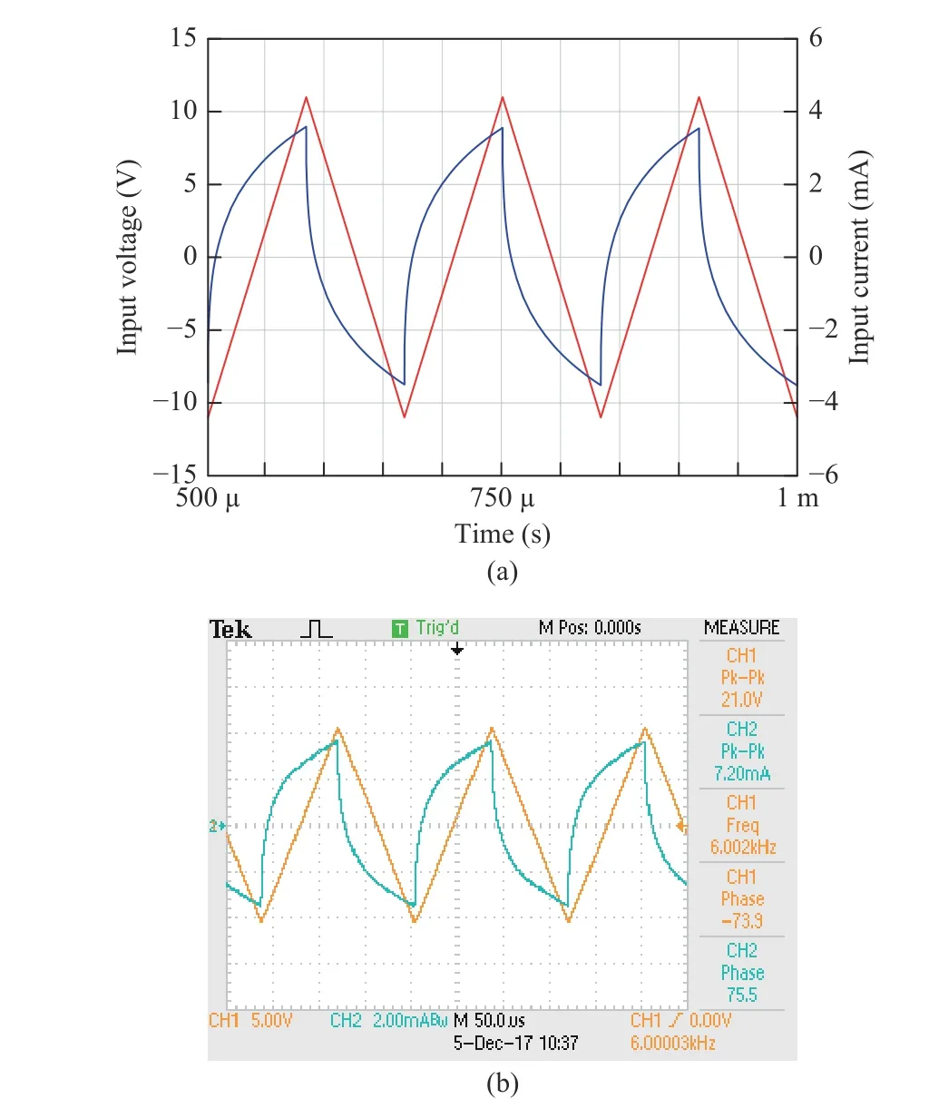
Fig.15. Experimental results with the triangular-wave voltage of 21 V peak-to-peak and 6 kHz frequency as the input: (a) simulation results of Multisim; (b) practical testing results.

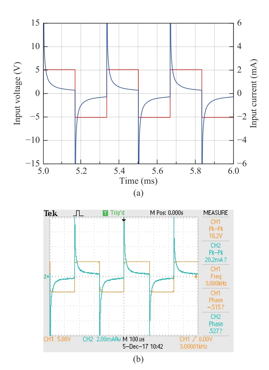
Fig.16. Experimental results with the rectangular-wave voltage of 10.2 V peak-to-peak and 3 kHz frequency as the input: (a) simulation results of Multisim; (b) practical testing results.

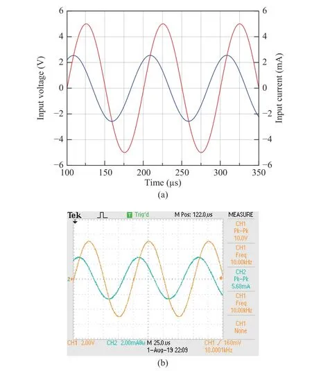
Fig.17. Experimental results with the sin-wave voltage of 10 V peak-topeak and 10 kHz frequency as the input: (a) simulation results of Multisim;(b) practical testing results.

operational order in the range 0<|µ|<1, but also obtain high order-stability characteristic and wider approximation frequency bandwidth. Approximation performance comparisons show that in the valid approximation frequency range there is no oscillation phenomenon in the frequencydomain characteristics of the impedance function calculated by the AHOSCWAFB. In addition, the approximation frequency bandwidth increases with the increase of the absolute value of the predistortion exponent. The design flow of the FACHOSCWAFB has also been described. As an example, a practical FACHOSCWAFB is designed and testified with electronic elements available on the market. Although operational amplifiers may be used, the FACHOSCWAFB shows excellent approximation performance and provides an alternative fractor in the future research.