Radiator Optimization Design for Planar Motors Based on Parametric Components

Ming Zhang， Qiaomu Xu， Rong Cheng， Leijie Wang and Xin Li

（State Key Laboratory of Tribology, Department of Mechanical Engineering, Tsinghua University,Beijing 100084, China）

Abstract: Focusing on the design problem of high-performance radiators for planar motors in the wafer stage of the lithography machine, a thermal-fluid coupling optimization scheme based on parametric solid components was proposed. The mapping method between component parameters and pseudo-density values was established. An analytical solution for the sensitivity of pseudo-density to component parameters was given. The conjugate heat transfer function with the shallow channel approximation term was solved through the pseudo-density information. In the optimization example, circular components were selected, and the position and the size of solid components were chosen as design variables. In order to eliminate calculation errors caused by pseudo-density,an optimized pseudo-density field was converted into the result based on parametric components.Compared to the reference motor radiator, the average surface temperature rise of the optimized water-cooling motor radiator is reduced by 22.4%, which verifies the feasibility and effectiveness of the proposed method.

Key words: motor cooling；conjugate heat transfer；parametric components；shallow channel approximation

The lithography machine is a crucial equipment in the integrated circuit manufacturing, in which the wafer stage is one of the key systems.In order to maximize the productivity of the lithography machine, the wafer stage operates at high speed and high acceleration, which requires large operating currents. Due to the limited design space of the radiator, the surface of the motor overheats and causes fluctuations in the environmental temperature. In order to reduce the influence of motor heating on the measurement accuracy of the optical system in the wafer stage, a high-performance water-cooling radiator must be introduced. Among the existing radiator optimization methods, the topology optimization method has been widely used in the thermalfluid coupling optimization problems.

In 2003, Borrvall[1]first proposed the Brinkman penalty term, and then Olesen[2]first introduced it into the Navier-Stokes equation. In 2009, Dede[3]first introduced the penalty term to solve a topology optimization problem based on the thermal-fluid coupling equations. Lee[4]pointed out that the penalty term may lead to instability in numerical calculations, resulting in intermediate density units and false flow paths as part of the optimization results. Scholten[5]pointed out that the density interpolation term and a high Reynolds number may increase the difficulty of the optimization convergence. To ensure the numerical convergence, the Stokes equation was applied instead of the Navier-Stokes equation. Haertel[6]adopted the inaccurate solid thermal conductivity in part of the optimization examples to avoid the generation of intermediate density elements and to ensure a stable convergence.

In order to alleviate the problems with numerical instability and divergence, the moving morphable components method for thermal-fluid coupling optimization proposed by Yu[7]in 2019 is adopted. Yu pointed out that compared to the traditional variable density method, the component method obtained optimization results with better heat dissipation performance. The fluid component parameters were used as design variables and the sensitivity of the objective function to component parameters was indirectly solved through pseudo-density. The component parameters and the size of the intermediate density region could be controlled within a reasonable interval. Therefore, the relevant numerical problems could be effectively alleviated.

To fulfill the actual design requirements of high-performance motor radiators in the wafer stage, an adjusted optimization method based on parametric components is proposed. First, the optimization results under uniform heat conditions in Refs.[8−10] show that most solid structures appear as small island-like regions, and the refined solid distribution characteristics can improve the heat dissipation performance. On the premise of having the same component number,compared to fluid components, solid components with simple geometry have fewer parameters,which can increase optimization speed. Therefore,in order to ensure both the structural complexity and calculation efficiency, solid components are selected as the optimization object. Secondly,the sensitivity of the pseudo-density to component parameters was calculated numerically using the finite difference method in Ref. [7], in which truncation errors[11]were inevitably introduced.The numerical error of the sensitivity calculation reduces the accuracy of the gradient optimization algorithm. Therefore, an analytical solution for the sensitivity of pseudo-density to component parameters is presented. In addition, because the flow channel of the water-cooling radiator is very thin, the two-dimensional thermal-fluid governing equations adopted in Ref. [7] cannot solve the velocity field under the specific boundary conditions. Therefore, a shallow channel approximation model is introduced into the governing equations. Finally, the result based on the pseudo-density information is converted into the result based on the component parameters to eliminate the calculation errors introduced by pseudo-density.

1 Thermal-Fluid Coupling Optimization Model Based on Parametric Components

1.1 Parametric solid component description method

Kotcioglu[12]compared the heat dissipation performance of solid components with different shapes, and pointed out that circular components were suitable for the design of water-cooling radiators. Therefore, the position and the size parameters of the circular solid components are selected as design variables here.

In order to establish the relationship between component parameters and pseudo-density, pseudo-density calculation points are uniformly selected in the domain of the optimization problem. Each point is first determined whether it corresponds to the solid or fluid material. For a circular component, the relative position of the pseudo-density point and thekth solid component can be determined by a single equation as

where (x′,y′) is the pseudo-density point coordinate, (xk,yk) is the component center coordinate,andrkis the component radius.

The maximum value of the relative position

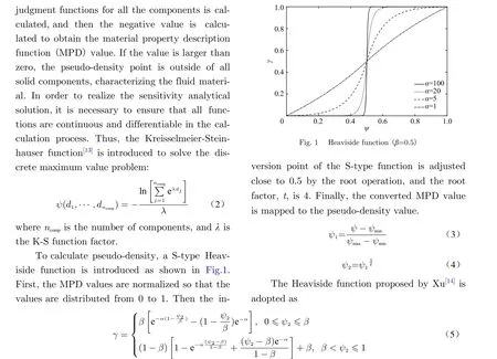
whereγrepresents pseudo-density,αis used to adjust the steepness of the S-type function, andβis used to adjust the inflection point position of the S-type function. As the parameterαincreases, the intermediate density transition layer at the fluid-solid boundary is narrower, and the optimization model is closer to the real model without intermediate density.

1.2 Thermal-fluid coupling control equation with the shallow channel approximation model

Based on the pseudo-density information,thermal-fluid coupling control equations with additional interpolation terms can be established. It is assumed that the properties of the fluid and solid materials (density, thermal conductivity,and heat capacity) and the fluid dynamic viscosity are independent from temperature. The fluid control equation is composed of the incompressible continuity equation and Navier-Stokes equation. The fluid control equation with the additional Brinkman penalty term is

wherepis the pressure,uis fluid velocity,μis dynamic viscosity,ρis density,εis the inverse permeability of the porous medium, anddzis the thickness of the radiator channel. The pseudodensity of the solid material is characterized by 0, and the pseudo-density of the fluid material is characterized by 1. The Brinkman penalty term is

whereqis the penalty factor,Lis the inlet width, andDis the Darcy number.

In the planar motor design problem, the space reserved for the water-cooling radiator is limited, and the thickness of the flow channel here is only 1 mm. The traditional two-dimensional Navier-Stokes equation results in a misleading calculation of the velocity field. Therefore, a shallow channel approximation model is introduced into the control equation through the COMSOL fluid simulation module.

The shallow channel approximation model can solve the fluid flow problem of thin channels.In such problems, the thickness of the flow channel is generally much smaller than the width of the flow channel, and the boundary layer has a great influence on the flow state. In order to solve such problems more accurately, the shallow channel approximation model can take the body force caused by the boundary layer into account[15].

In the heat conduction control equation as solid isotropic material with penalization (SIMP)is adopted as the material interpolation method:

where f represents fluid, s represents solid,nρis the penalization factor of density,nkis the penalization factor of thermal conductivity,ncis the penalization factor of heat capacity,kis the thermal conductivity,cis the heat capacity under constant pressure,Qis the heat flux, andTis the temperature field.

1.3 Optimization objective and constraints

The optimization objective is the average temperature of the design domain, with a 95%fluid volume fraction constraint.

To ensure that the optimization space is within the design domain, the upper and lower limits of the position design variables are introduced. To avoid local overheating caused by oversized solid components, a maximum on size design variables is introduced as a constraint. If the component size is close to zero, it has a lesser effect on the heat dissipation performance of the optimized structure. However, such an overly refined feature increases the manufacturing difficulty. Therefore, a minimum value constraint on the size variables is introduced.

The values of relevant parameters in the optimization algorithm are shown in Tab.1.

Tab. 1 Optimization parameters

The optimization problem can be described as follows:

wherefis the objective function,gis the fluid volume fraction constraint function, andVfis the maximum fluid volume fraction.

The optimization algorithm flow is shown in Fig.2.

Fig. 2 Flow chart of optimization algorithm

1.4 Sensitivity analysis

The MMA algorithm proposed by Svanberg[16]is adopted here. The algorithm is a typical gradient algorithm, so the sensitivity analysis of the objective and the constraint is required.

To obtain the sensitivity of the objective function to the component parameters, the calculation is divided into two steps: the first step is to calculate the sensitivity of the objective function to pseudo-density through the adjoint method. The second step is to calculate the sensitivity of pseudo-density to the component parameters.

The design variablex1is taken as an example to show the sensitivity calculation process:

wherenγis the number of the pseudo-density calculation points.

The sensitivity of the objective to component parameters can be decomposed into three steps:

① Gradient of pseudo-density to MPD:

where

② The gradient of MPD to the relative position function of thekth component:

③ The gradient of the relative position function to the component parameter.

All the above steps are analytically calculated, and the related functions are continuous and differentiable. Thus, the accuracy of the sensitivity analysis is ensured.

The sensitivity analysis of the constraint function to the component parameters also adopts the above method:

2 Numerical Example

2.1 Optimization model

The two-dimensional optimization problem is studied here. As shown in Fig.3, the geometric model consists of the inlet, the outlet, and the design domain. Since the design space of the planar motor is strictly limited, the inlet and the outlet are on the same side of the design domain,and the widthLof the inlet is 10 mm.

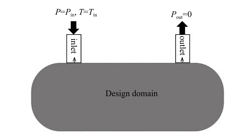
Fig. 3 Two-dimensional optimization model and boundary conditions

The laminar inflow condition is applied at the inlet, and the relative pressure is 50 Pa. The inflow temperature is 293.2 K. The laminar outflow condition is applied at the outlet, and the relative pressure is 0 Pa. The other boundary conditions are adiabatic and no-slip. The heat flux is 0.4 W/cm2, assuming that the heat source is uniform throughout the design domain. The properties of the fluid and solid materials are shown in Tab.2.

Tab. 2 Properties of the fluid and solid material

The characteristic Reynolds numberR(inflow Reynolds number) of the model is 325

wherevinis the average inlet flow velocity. Therefore, this example is a typical laminar flow problem.

As shown in Fig.4 and Fig.5, an initial distribution of approximately uniform solid components is selected. The number of solid components is 60, and each component has 3 design variables(abscissa, ordinate, and radius) that characterize the position and the size. In total, the optimization model has 180 design variables. The initial value of the objective function, which is the average temperature of the domain, is 308.2 K.

Fig. 4 Initial distribution of solid components

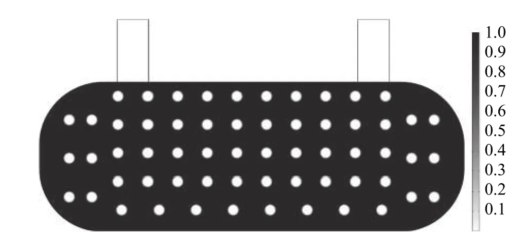
Fig. 5 Initial distribution based on pseudo-density description

In order to obtain the sensitivity information, a pseudo-density description method is introduced in the optimization calculation, so there is an intermediate density transition layer at the boundary of each component. This layer has a certain blocking effect on the fluid flow, which is equivalent to increasing the component size, so the component size is taken to a smaller value in the optimization step. In this example, the radius ranges from 1.0 mm to 2.5 mm, and the initial radius of all the components is 1.75 mm.

2.2 Optimization result based on pseudo-density description

It can be seen from Fig.6 that some solid components gradually intersect or overlap during the iteration process. The intersection of the solid components is equivalent to the geometric change of the components, which increases the optimization searching space of the algorithm.Some components have a similar effect on the flow channel shape, resulting in the overlap of some solid components, which means the number of the selected solid components is in excess and sufficient in this example.

Fig. 6 Intermediate iterations

The MMA algorithm is a gradient-based algorithm. Due to the high complexity of the nonlinear and multi-peak thermal-fluid coupling optimization model, the MMA algorithm is not able to find the global optimal solution based on gradient information. Therefore, the optimization result of this model inevitably falls into a local optimal solution.

The convergence criterion is that the objective difference between the two iterations is less than 0.01 K. After 29 iterations, the objective converges, and the objective function value drops to 303.4 K. The convergence history is shown in Fig.7.

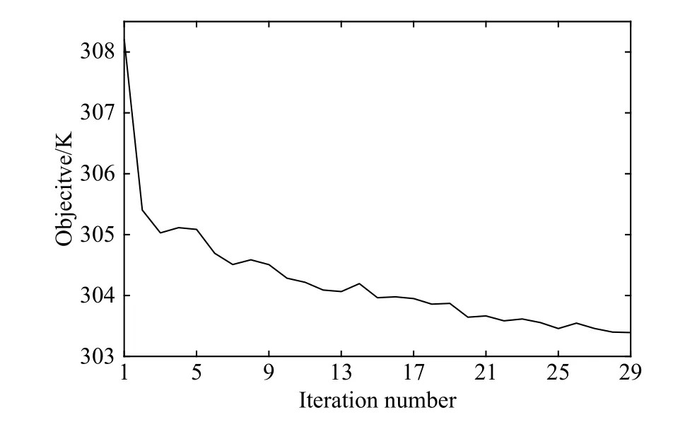
Fig. 7 Convergence history

The value of the optimal fluid volume fraction is unknown before optimization, but it should be ensured that the fluid volume fraction constraint is greater than the optimal value. As shown in Fig.8, the optimal fluid volume fraction is 91.5%, which is less than the constraint value of 95%. Therefore, the 95% fluid volume fraction constraint is reasonable.

Fig. 8 Pseudo-density distribution of optimization result

The temperature field and the velocity field based on pseudo-density description are shown in Fig.9 and Fig.10. The effects of the solid regions on the temperature distribution and the flow state are as follows: ① the number of branch channels is large, and the mainstream channel at the entrance extends to the lower left, ② most solid components are distributed at the lower right side of the inlet, forming a complex branch channel network, which effectively dissipates most heat, ③ some components are arranged closely, forming narrow channels to increase the local flow velocity, ④ multiple flow channels converge to form a wide flow channel along the bottom wall, which improves the heat dissipation at the bottom, ⑤ the arrangement of the top components minimally allows water to pass through the shortest channel, ⑥ some components are arranged side by side, which is beneficial to the formation of long flow channels, ⑦ high-temperature areas are concentrated in the right design domain at the end of the flow channel due to the inlet and the outlet being on the same side.

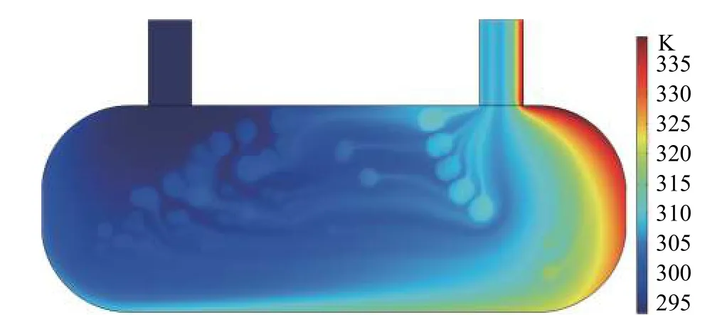
Fig. 9 Temperature field based on pseudo-density description

Fig. 10 Velocity field based on pseudo-density description

2.3 Optimization result based on parametric component description

The position and the size of the intermediate density produced by traditional topology optimization cannot be controlled, so it is difficult to propose a suitable post-processing method.However, a controllable intermediate density layer is artificially introduced by mathematical means here. This layer is evenly distributed at the component boundary. By decreasing the thickness of the transition layer, the influence of the layer on the flow characteristics and temperature distribution can be reduced. In order to eliminate the calculation errors caused by pseudo-density description and obtain accurate temperature and velocity distributions, the layer near the solid side is considered solid to simulate the blocking effect, and the layer near the fluid side is considered fluid to simulate the liquidity.

The varying intermediate density threshold corresponds to different solid component sizes.The calculation result with different size conditions is shown in Tab.3. The data shows that as the component size increases, the objective function gradually decreases. Here, the radius range is increased to 1.25–2.75 mm, and the corresponding objective function is 303.6 K, which is close to the calculation result based on pseudo density.

Tab. 3 Objective values with different size conditions

The parameterλdetermines the accuracy of the maximum value operation, andλis 20 in this model. The maximum value operation of the first iteration is given as an example here. The direct discrete result of all MPD values are compared with the K-S function result. The MPD values calculated by the two methods both range between – 1.725 0 and 13.623 0. The maximum calculation error of MPD values is 0.062 2, and the average calculation error is 4.658 2×10−4.Compared to the maximum value, the calculation error is rather small. According to the optimization result based on the pseudo-density description and the optimization result based on the parameterized component description, the KS function and Heaviside function only produce an error of 0.2 K for the optimal value of the objective function. Therefore, the value of parameterλis reasonable in this example.

As shown in Fig.11 and Fig.12, the optimization results based on the pseudo-density description and parametric component description have similar flow channels and temperature distribution characteristics. The result based on the pseudo-density description has a lower average temperature in the design domain, indicating that the characteristics of the intermediate density units are conducive to further improving heat dissipation performance. However, such micro channels are not able to be fabricated in the engineering setting, so the improved heat dissipation performance has no physical relevance.

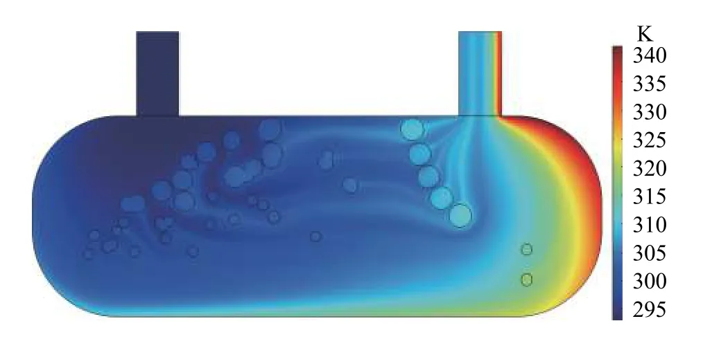
Fig. 11 Temperature field based on parametric component description

Fig. 12 Velocity field based on parametric component description

2.4 Three-dimensional simulation comparison

In order to verify the heat dissipation capability of the optimized motor radiator, a reference motor radiator used in engineering practice was introduced. Fig.13 and Fig.14 respectively show the optimized radiator structure and the reference radiator structure. The boundary conditions in the three-dimensional simulation are consistent with those in the two-dimensional optimization problem.

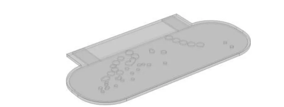
Fig. 13 Three-dimensional flow channel of optimized radiator

Fig. 14 Three-dimensional flow channel of reference radiator

The design principle of sufficient and uniform flow is adopted in the reference radiator.The reference model has 4 flow channels designed from the inlet to the outlet. The baffle width between the flow channels is 0.5 mm, and the width of the baffle in the center channel is 2 mm. Because the outside of the design domain faces greater heat dissipation pressure, the width of the outside channel is larger than the inside channel.

In the design of the planar motor radiator,the thermal performance index is considered the rise in surface temperature. As shown in Fig.15 and Fig.16, the average temperature rise in the upper surface of the reference radiator is 11.6 K,and the average temperature rise in the upper surface of the optimized radiator is 9.0 K. The optimized radiator reduced the average temperature rise by 22.4% compared to the reference radiator. The maximum surface temperature of the reference radiator is lower. However, because there is no short channel design, by the time fluid reaches the right side of the design domain,the fluid heat dissipation capacity has already decreased substantially, and the high temperature area has increased substantially. Therefore, the average surface temperature rise of the reference model is higher than the optimized model. The feasibility and efficacy of the proposed optimization method in the design of planar motor radiators are proved by the above comparison.

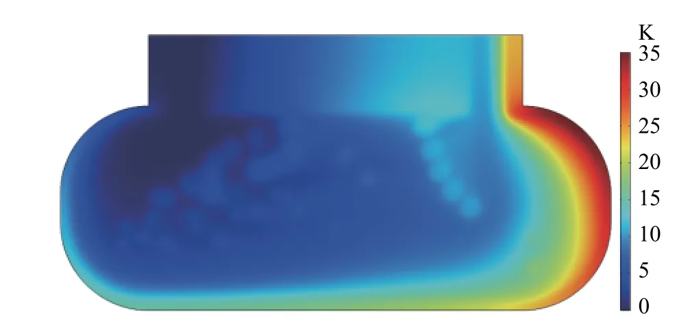
Fig. 15 Surface temperature rise of optimized radiator

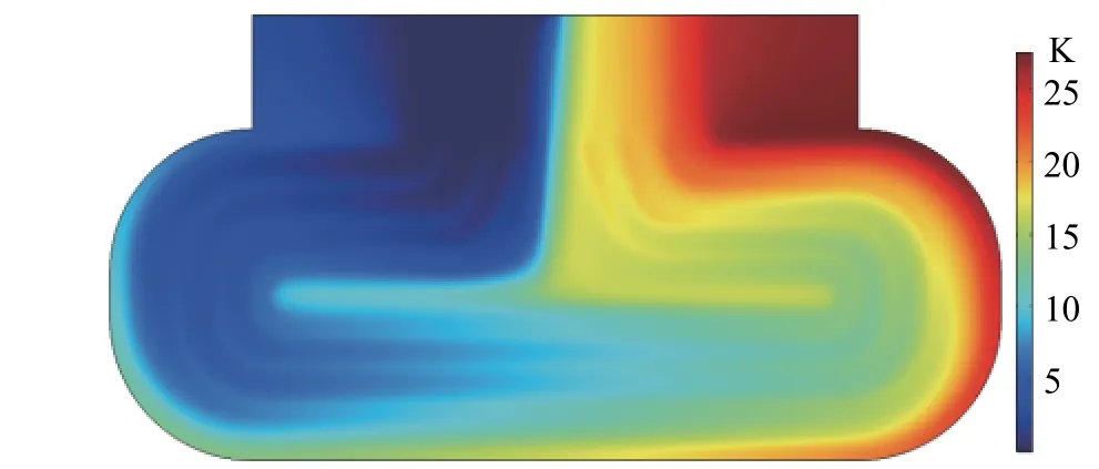
Fig. 16 Surface temperature rise of reference radiator

3 Conclusion

Oriented to the design requirements of the high-performance water-cooling radiator for planar motors, the solid component parameters are chosen as design variables. The shallow channel approximation model is introduced into the thermal-fluid coupling equations, and an analytical solution for determining sensitivity of the pseudo-density to component parameters is given. The pseudo-density description is indirectly introduced to realize the optimal design of the radiator based on parametric components. The 3D simulation comparison proves that the optimized radiator effectively improves the cooling performance of the planar motor. The circular solid components are selected as the optimization objects here. Future models will entail the more structurally complex solid components. In a future work,the optimized radiator will be manufactured to experimentally verify the models develop in this work.