Reconstruction of hollow areas in density profiles from frequency swept reflectometry

Rennan B MORALES , Stéphane HEURAUX , Roland SABOT,Sébastien HACQUIN,5, Frédéric CLAIRET and the Tore Supra Team

1 United Kingdom Atomic Energy Authority, Culham Centre for Fusion Energy, Culham Science Centre,Abingdon, Oxon, OX14 3DB, United Kingdom

2 IJL, UMR CNRS, University of Lorraine, BP50840, Nancy, F-54011, France

3 Institute of Physics, University of Sao Paulo, Sao Paulo 05315-970, Brazil

4 IRFM, CEA, Cadarache, F-13108 Saint-Paul-lez-Durance, France

5 EUROfusion Programme Management Unit, Culham Science Centre, Culham OX14 3DB, United Kingdom

Abstract The standard density profile reconstruction techniques are based on the WKB approximation of the probing wave’s phase,making them unable to properly reconstruct blind areas in the cut-off frequency profile. The reconstruction suffers a significant immediate error that is not rapidly damped. It is demonstrated that even though no reflections occur inside the hollow region causing the blind area,the higher probing frequencies that propagate through it carry information that can be used to estimate its properties. The usually ignored full-wave effects were investigated with the use of full-wave simulations in 1D, with special attention paid to the frequency band where they are dominant. A database of perturbation signals was simulated on five-dimensions of parameters and an application of the database inversion was demonstrated for a magnetic island in a Tore Supra discharge. The new adapted reconstruction scheme improved the description of the density profile inside the hollow region and also along 10 cm after it.

Keywords: FM-CW reflectometry, profile reconstruction, reflectometry density profile, hollow profile, blind area(Some figures may appear in colour only in the online journal)

1. Introduction

The frequency-modulated continuous-wave (FM-CW) reflectometry diagnostic is a well established technique for density profile measurement with successful implementations on various medium and large size tokamaks, such as DIII-D [1],Tore Supra [2, 3], ASDEX Upgrade[4, 5] and JET[6]. Even though there have been significant improvements in the reflectometry hardware design [2, 7] and data extraction techniques [5, 8, 9] over the last two decades, the measured density profiles on fusion experiments still require further improvements in the data analysis front in order to improve the accuracy of the reconstructed profile. As an example of a demanding application,the low field side (LFS) reflectometer being built for ITER has as its first operation priority to achieve a minimum radial accuracy of 5 mm [10]. Improving the accuracy on the reconstructed density profile also improves the accuracy of extracted parameters for fusion studies such as confinement,transport, MHD instabilities and turbulence.

The data analysis for FM-CW profile reflectometry can be divided into three topics: the initialization technique as initially investigated in [11]; the recursive profile reconstruction algorithm as originally proposed by Bottollier-Curtet[12] with minor revisions in [13, 14] and a thorough review with some improvements in [15]; and the reconstruction of blind areas, as focused in this contribution.

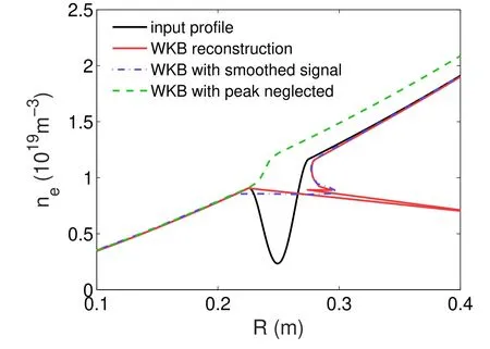
Figure 1. Synthetic example of input versus reconstructed density profiles with a blind area. The profile was reconstructed with the standard Bottollier-Curtet algorithm and a constant correction, as in[13–15], using three different treatments in the phase signal. The radial axis is defined from zero at the plasma edge and increasing towards the plasma center.

Both O-mode and X-mode density profile reconstruction techniques rely on the assumption of a monotonic cut-off frequency profile.However,there are many plasma perturbations that introduce hollow areas in the cut-off frequency profile,breaking the aforementioned assumption. Inside these hollow areas, the probing microwaves exhibit no specular reflections and thus they are refereed to as blind areas. Even though no reflection occurs inside the blind areas, the higher probing frequencies that propagate through them carry information related to its properties. For isolated perturbations, the perturbation signature in the reflectometer signal is related to the size and shape of the perturbation. In this contribution, large perturbations are considered, which are out of the Born approximation validity and the probing electric field over the perturbation is no more similar in magnitude to the unperturbed case. This situation can occur during massive gas and pellet injections [16], MHD activity [17] and in hollow profiles that emerge during the initiation of heating systems [18] or even due to relativistic effects [19].

If the reconstruction method does not incorporate identification and reconstruction tools for large blind regions, big discrepancies appear in the reconstructed profile.An example is shown in figure 1 using a simulated phase under the WKB approximation as the input signal and profiles typical of Tore Supra with a low magnetic field strength of 2 T at the plasma center.

It is clear from figure 1 that the unmodified standard reconstruction algorithm is unable to reconstruct the density perturbation. Furthermore, if the oscillations are smoothed,the perturbation can be neglected entirely, or even worse, a radial shift can be introduced in the reconstructed profile after the perturbation if the time-of-flight jump is filtered out,which is the case for the dashed green line in figure 1.

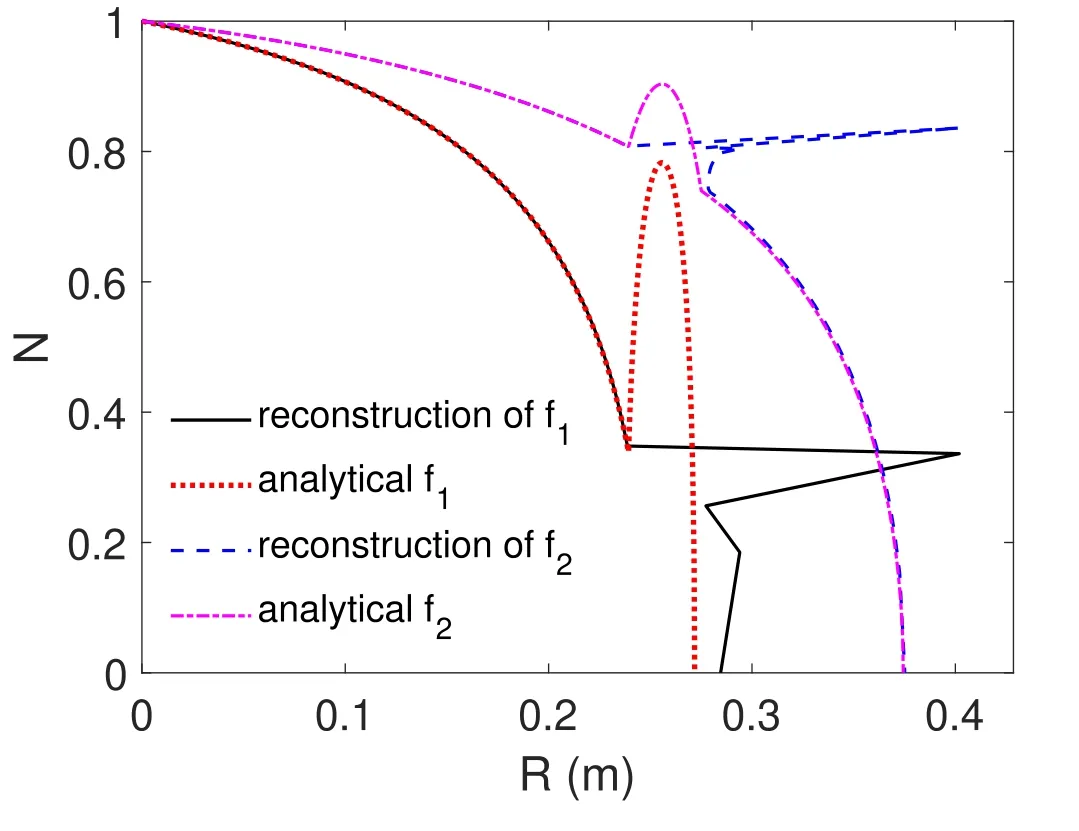
Figure 2.Refractive index profiles for two different probing frequencies, f1 and f2, corresponding to two different cut-off positions, at 0.272 and 0.375 m. The analytical cases correspond to the refractive index calculated along the input analytical profiles,whereas the reconstruction cases correspond to a simulated profile reconstruction of these analytical profiles using the standard algorithm. The radial origin is at the plasma edge starting with zero density (hence N(0)=1) and increasing towards the plasma center.A sine perturbation was introduced at the position of 0.26 m with a 4 cm width and a depth in the cut-off profile of 10 GHz. The conditions simulated correspond with typical Tore Supra parameters:plasma radius of 0.72 m and at the plasma core a magnetic field strength of 2.5 T and electronic density of 6×1019 m-3.

The density profile reconstruction algorithms developed in [14, 15] for X-mode reflectometry are based on linear integrations of the refractive index, except for the last integration step in[15],where the shape of the refractive index is optimized based on the local plasma parameters. Due to a sharp change of the refractive index near the cut-off position,the shape of the last integration step is the main factor that dictates the accuracy of the reconstructed profile. As explained in [15], the trapezoidal integration over all radial steps before the final radial step is always more accurate than the integration on the last step for smooth monotonic density profiles, unlike the profiles treated in this paper. Such disparity was initially predicted in [14] with the observation of refractive index profiles similar to those displayed in figure 2.

The inaccuracy of the trapezoidal integration causes large discrepancies on the reconstructed density profiles observed in figure 1. As can be seen in figure 2, a probing frequency just above the blind area,f1,undergo abrupt changes in the refractive index path, which leads to a poor discrete description of the correct refractive index along the perturbation during the reconstruction process. Specially on the first probing frequency that crosses the valley without being reflected, in the standard reconstruction algorithm, the refractive index is incorrectly assumed to monotonically decrease from before the valley until it is equal to zero. This big initial discrepancy in the phase data overshoots this reflection position far inside the profile,as observed.As the probing frequency is increased, the perturbation on the refractive index path diminishes and the error caused in the reconstructed reflection position decreases, as can be observed for the probing frequency f2.

Even though the probing microwaves are not reflected inside the blind region, there is information to be explored from the higher probing frequencies that propagate through the perturbation. The parameters necessary to describe a perturbation are: the perturbation width; the perturbation depth; and the perturbation shape. For simplicity, the first perturbations investigated have a well known shape and width and are inserted in a region with linear cut-off frequency profile, fcut, which can be either fpewhen probing with O-mode or fRif probing with the right-hand X-mode.Ideally,the entire density profile is first reconstructed in an unperturbed state, and as the perturbation appears, the additional perturbation in time-of-flight is used to infer the valley depth.

2. Reconstruction of blind areas from a database of perturbation signatures

The density profiles of the blind areas can be reconstructed by inverting a database of perturbation signatures in the time-offlight signal.Various perturbations were investigated with 1D full-wave simulations(4th order Runge–Kutta wave equation solver [20, 21]) in [22]. It was observed that the full-wave effects simulated in 1D (tunneling, wave-trapping, scattering and interference)were restricted to a probing frequency band of about 1 GHz around the time of flight jump over the blind area. This frequency band is also marked by a drop in the signal amplitude, which indicates that the full-wave effects have lower amplitude than the cut-off reflection and therefore are only observable when the power being received from the cut-off reflection decreases. This conclusion refers mostly to the scattering and wave-trapping effects, whereas the wave tunneling into the blind region is the effect causing the strong decrease of the detected amplitude around the probing frequency that jumps over the blind area. As long as a corresponding experimental signal is treated outside of the bandwidth affected by full-wave effects (the bandwidth of reduced amplitude), the WKB approximation provides a suitable description of the experimental time-of-flight signal.In this case, the database can be formed by WKB simulated signals,which are significantly faster and simpler to compute compared to their full-wave counterparts.

The WKB compatible signals computed for the database are the excess time-of-flight caused by the perturbation along the unperturbed profile after the perturbation. Only with this approach it is possible to dissociate these database perturbation signals from the vast possible profiles that can exist before the perturbation. In this circumstance, to account for this general approach and also for a vast application domain(including both O and X-mode probing captured by the variable fce), the database of time-of-flight signals (time-offlight vs probing frequency after the perturbation) is computed over the following free parameters: (shape, width,fce,∇fcut, fend).

A schematic of the algorithm to reconstruct a blind area from a database is presented in figure 3. The numbers 1–7 represent all steps to reconstruct a blind area once the unperturbed data has been saved from a previous frequency sweep. Ideally, for maximum compatibility, the unperturbed data comes from the last sweep where a blind area was not detected and the cut-off profile after the perturbation is assumed to not have changed significantly. Each step numbered on the algorithm diagram is explained on the subsections below.

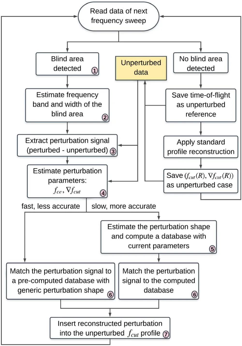
Figure 3.Algorithm of a blind area reconstruction scheme.

2.1. Detection of a blind area

As the cut-off moves with the increase of the probing frequency, at one point the cut-off location will jump from before the blind area to after the blind area,causing a jump to appear in the time-of-flight signal. Before this jump, the probing waves start to tunnel into the blind area,and can even be trapped for a short time inside this cavity. By the time these probing waves return to the detection antenna,this time gap also causes a dip in the detection amplitude signal. The combination of the amplitude dip with the jump in time-offlight is a clear indication for the presence of a blind area.This feature was verified in many simulations included in[22]and in the experimental signals discussed in section 3.

For an automatic detection of the presence of blind areas,a threshold can be set for both the amplitude drop and the time-of-flight jump. The detection is only confirmed when both conditions are satisfied.Furthermore,the exact threshold can be fine tuned to be greater than the current fluctuation level and signal-to-noise ratio to avoid false detections.

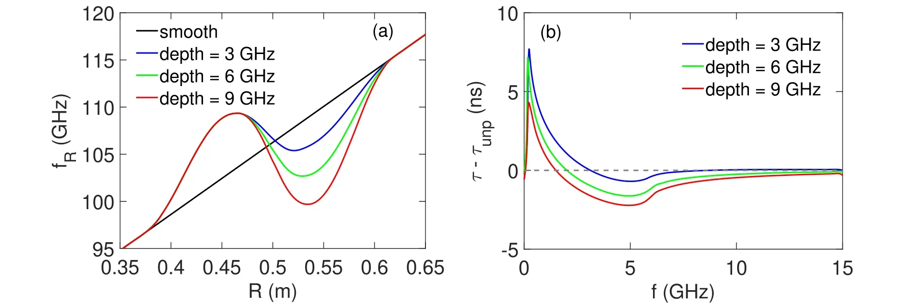
Figure 4.(a)25 cm long bump-valley perturbations added on a linear cut-off profile.The valley has a varying depth while the bump is kept with a constant height of 6 GHz.(b)The corresponding simulated spectrogram time-of-flight signals additional to the unperturbed case and with the frequency axis starting at the top of the bump section at 110 GHz.

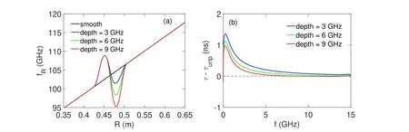
Figure 5.(a) Cut-off profile of 9 cm long bump-valley perturbations added on a linear fcut profile. The valley has a varying depth while the bump is kept with a constant height of 6 GHz. (b) The corresponding simulated spectrogram time-of-flight signals additional to the unperturbed case and with the frequency axis starting at the top of the bump section at 110 GHz.

2.2. Estimation of the frequency band and width of the blind area

The perturbation width (which also gives the frequency band in the cut-off profile and probing frequency)is defined by the end location minus the starting location of the perturbation.The beginning of the blind area and its first probing frequency comes directly from the standard reconstruction scheme up to the blind area. The end of the perturbation is found by associating a feature in the perturbation time-of-flight signature to the end of the perturbation. Once this probing frequency is determined,the end of the perturbation is found by taking the position in the reconstructed unperturbed profile that corresponds to the same probing frequency.Figures 4 and 5 show two cases to observe the signature that marks the end of the perturbation. In this circumstance, the probing waves are injected from the left at R=0 and propagate to the right.The chosen examples are double perturbations because the interpretation of them clarifies all single and double perturbation cases. The examples in figure 4 are equivalent to a single valley perturbation because the end of the perturbation is exposed, and the examples in figure 5 have a positive perturbation obstructing the end of the perturbation.

Equivalently to a single valley case, the additional timeof-flight in figure 4, right, exhibits a minimum marking the end of the perturbation at 5 GHz after the top of the bump section. This feature is not a coincidence and has been observed for many different perturbations. One interpretation that yields this minimum is the observation of time-of-flight change due to the change in the cut-off gradient. The higher the gradient, the faster the group velocity goes to zero at the cut-off location, resulting in a decreased time-of-flight inside the valley until it goes back to the unperturbed case.

The second case, corresponding to figure 5, represents cases where the end of the perturbation is not exposed because the prior bump is high enough such that the probing waves are reflected in the bump and when going above, they already reflect past the perturbation end point. In such cases,there is no clear indication of the end of the perturbation and there are two methods to estimate the end of the perturbation:(1) the perturbation is assumed symmetric, i.e. the width of the combined perturbation is equal to twice the width of the positive perturbation (or four times the first quarter of the perturbation, which is conventionally measured and reconstructed);or(2)the perturbation end is assumed to be probed at the first probing frequency that travels over the bump and through the valley. If there is no information to distinguish between these two cases, one can rebuild the perturbation with each case and assume the perturbation end to be within these two limits with an associated error bar.

An additional feature from figures 4 and 5 is the magnitude of the additional time-of-flight compared to the valley depths. As the valley decreases, the additional time-of-flight increases. They behave this way because the probing waves travel much slower (lower refractive index and lower group velocity)while propagating in a region with cut-off frequency very close to the probing frequency. If such region is large,the next probing frequencies can even return to the antenna before the lower probing frequencies,which causes frequency mixing. This effect is pronounced at lower refractive indexes near the cut-off location as can be seen by the refractive index behavior in figure 2. This effect also dictates the approach to estimate fcefor the database, as discussed in section 2.4, and the reflectometer response to different perturbation shapes,as elaborated in section 2.5.

2.3. Estimation of the perturbation signal

Once the unperturbed time-of-flight and the perturbation width and probing band have been estimated,the perturbation signal can be obtained by taking the measured perturbed timeof-flight minus the unperturbed time-of-flight, starting at the end of the perturbation (perturbation end found as explained above in section 2.2). This signal represents the additional time-of-flight caused by the perturbation over the following unperturbed section.

2.4. Estimation of the parameters fce and ∇fcut

The estimations of the parameters fceand ∇fcutare straight forward once the perturbation width has been estimated over the unperturbed profile. The parameter ∇fcutcomes directly from calculating the gradient over the two points of the fcutprofile (start, end), and the fceparameter comes from the equilibrium reconstruction. As it was noted in [22], the additional time-of-flight from a perturbation comes mostly from the higher cut-off frequency section of the blind area.Therefore,for simplicity,the used fcevalue can be taken from the end of the perturbation when it is exposed, or from the beginning of the perturbation when it is not exposed.

2.5. Estimation of the perturbation shape

As shown in the algorithm diagram (figure 3), the shape estimation step can either follow a slower more accurate reconstruction route or be skipped entirely for a faster less accurate reconstruction when the reconstruction speed has priority.

In the fast case, the perturbation signal database is precomputed with a generic shape and applied to any perturbation detected. When a generic shape is used, the precision of the reconstruction tends to be lower. However, the generic shape can be chosen to target expected perturbations if there is any prior information about the expected shape, and these cases are fast and accurate. If following the generic route, a suggested shape for a blind area can be a cosine function from 0 to π. A good feature of this shape is the zero derivative at the start and end of the valley, which allows for the subtraction from the unperturbed profile without causing any derivative discontinuity in the resulting profile.

The slower route is to be followed when the reconstruction accuracy has priority and there is information about the shape of the blind area within the discharge being analyzed.In principle, it is possible to seek details from the fullwave effects in the blind area signal that indicate the perturbation shape. However, these effects were observed in [22]from 1D simulations and a study of them in 3D would be necessary to verify the validity of this approach. The 1D model is expected to specially enhance their amplitude response. Furthermore, the extraction of this information in today’s experimental signals is practically unfeasible due to the mix of all full-wave effects, fluctuations and instrumental noise.The alternatives are to either resort to the precomputed database route assuming a shape information from other studies of the perturbation in focus (be it numerical or theoretical), or to use a shape reference from data in the current discharge. One example is to determine the valley shape from a positive perturbation before the valley in cases where the double perturbation can be assumed symmetric, as done and justified in section 3.

A comprehensive study of the impact of different valley shapes on the database signals is too extensive to be incorporated in this publication. Nevertheless, the impact of the shape skewness and kurtosis has been investigated in [22]. It turns out that the skewness of the blind area is only a minor second order effect compared to the kurtosis. The skewness effect was tested in a perturbation where the start and end of the valley had the same cut-off frequency. Therefore, the effect can only be caused by a different value of fceat these two points.Moreover,since already mentioned that the excess time-of-flight signal always has significantly more contribution coming from the higher cut-off frequency region, if the fceparameter in a blind area is taken from the highest cut-off frequency region,this skewness effect decreases even further.Thus, the vast majority of reconstructed blind areas end up being symmetrical because the reflectometer cannot distinguish between different skewness. The skewness effect is expected to be non-negligible only when the start and end of the perturbation lie in very similar cut-off frequencies and the∇fcein the region is very high (e.g. if probing from the high field side). In such specific cases, the value of the parameter fcecannot be assumed constant over the perturbation and the database would need to include the additional parameter ∇fce.

The perturbation kurtosis, on the other hand, was found to have a first order influence on the perturbation excess timeof-flight.The test was performed by varying the exponent n in a cosnperturbation shape. The higher the kurtosis (n increases), the higher is the additional time-of-flight due to the perturbation because the probing waves take longer to propagate through the areas closer to the respective cut-off frequency. More specific details of the shape comparisons mentioned can be found in[22].The following results in this paper are not strongly affected by this dependency because the experimental application investigated has a well-defined perturbation shape.Future research on this topic will focus on worse defined perturbation shapes and an error bar is foreseen to accommodate a range of possible perturbation shapes.

2.6. Finding the perturbation depth by comparison to the database

Regardless of the fast or slow path followed with respect to determining the perturbation shape, the following step is to compare the experimental excess time-of-flight signal to the signals stored in the database for the current set of parameters and varying depth. The best signal match directly indicates the associated perturbation depth.Moreover,a depth error bar can be extracted based on the match confidence that is dictated by the experimental signal noise level.

2.7. Applying reconstructed perturbation into unperturbed profiles

The perturbed cut-off profile is determined starting from the unperturbed cut-off profile and subtracting the perturbation found in the previous step. This approach eliminates the discrepancy caused on the reconstructed profile just after the blind area.

This section completes the description of the blind area reconstruction algorithm as depicted in figure 3. The next section elaborates on the intrinsic accuracy of the database reconstruction scheme and next in section 3, the example experimental blind area reconstruction uses the noise level in the experimental signal to determine the depth error bar.

2.8. Accuracy of database reconstruction

An initial generic database was precomputed for a simple cosine shaped valley and a broad range of all parameters(fprob,fce,∇fcut,width,depth),including coverage for both X and O-mode since the fcedomain starts at zero. The database inversion procedure was tested with great success in a noisefree synthetic example using this precomputed database to describe cosine shaped perturbations. As covered in detail in[22], it also demonstrated how a single database can accommodate a broad range of plasma conditions and it was also used to infer the dependencies of the reconstruction accuracy across the full database domain. As expected, the reconstruction accuracy decreases when the perturbation signal is smaller, as is the case for the highest cut-off gradients and widths. However, the intrinsic database accuracy is not enough to know the reconstruction accuracy. In practice, the biggest contribution to the inversion accuracy is expected to come from the precision of the estimations of the perturbation width, gradient, the unperturbed signal and the experimental noise level. In conclusion, there is a large number of parameters that can influence the final accuracy, and each application has specific parameters which are relevant and result in different bottlenecks in each case. Therefore, the reconstruction in experimental cases must be accompanied by an analysis of the relevant parameters specific to that application and error bars can be estimated from the available spread of the relevant parameters.

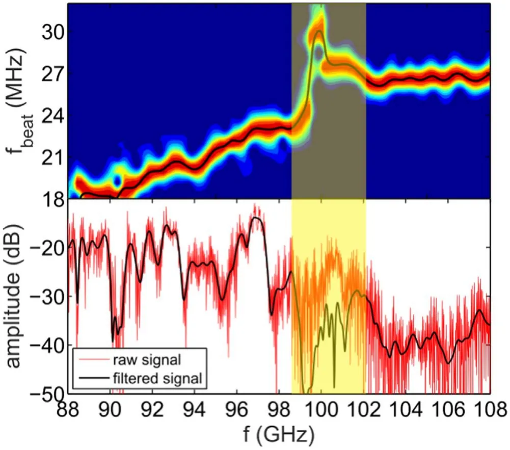
Figure 6.Beat frequency and amplitude signals around the perturbation to be investigated. Only a broad band-pass filter(40 MHz wide)was applied to remove reflections that were far from the main branch. Tore Supra discharge 32 029 at t=3.0037 s,acquired with a 20 μs sweeping time and a sampling rate of 100 MHz.The marked zone in yellow represents the band dominated by full-wave effects.

3. Experimental demonstration of detection of a blind area and its reconstruction

The chosen first experimental application of the database inversion method was a magnetic island observed in Tore Supra. The perturbation being investigated builds up from previous observations of MHD activity with reflectometry[23, 24]. In this circumstance, the focus is on the reconstruction of the magnetic island on the q=2/1 rational surface, as located by the equilibrium code [24]. The used beat frequency and amplitude signals around the perturbation are displayed in figure 6.

Figure 6 shows a perturbation signature around the probing frequency of 100 GHz on the beat frequency and amplitude signals which are caused by a blind area to be reconstructed. The indicator of a blind area is the discontinuity on the spectrogram paired with a strong drop in the amplitude signal, as foreseen in [22]. Only a broad (40 MHz wide)band-pass filter was applied in the beat frequency signal and the selected window size for the spectrogram was 90 points to ensure that the spectrogram captures the fast changes in beat frequency (or equivalently in time-of-flight). For this specific application, the frequency of appearance of the perturbation due to the magnetic island is easily defined from observing the time-of-flight signal. The signal used for the reconstruction,as given in figure 6,corresponds to the biggest perturbation signature that is obtained when probing across the island O-point.On the other hand,the unperturbed signal is readily available before or after half rotation of the magnetic island,while probing through the island X-point.Figure 7 illustrates the perturbed time-of-flight signal at the O-point compared to the smoothed reference unperturbed signal in white corresponding to probing the X-point.

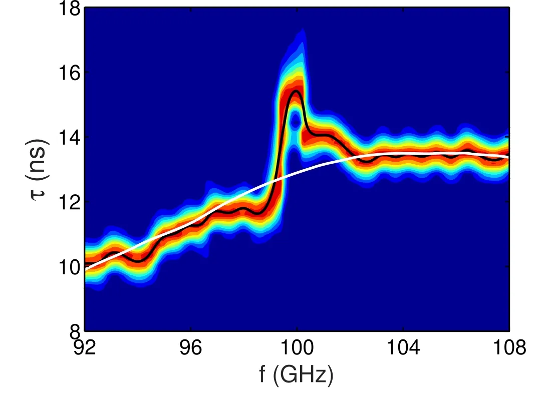
Figure 7. Time-of-flight signal around the perturbation of interest compared to the reference unperturbed case in white. Tore Supra discharge 32 029, with the perturbation at t=3.0037 s and the reference unperturbed case at t=3.0033 s.

Note that the resulting perturbation signal does not necessarily have the same shape as the signals illustrated in figures 4 or 5. It would be very similar if comparing single perturbations, but double perturbations are too complex and not always have the same signal shape.Specially in this case,all conditions are different (shape, fce, ∇fcut, width, depth).The variation of these parameters in a double perturbation will change the signal shape significantly. This behavior is precisely the reason for using the most general database (full time-of-flight signals) instead of fitting the time-of-flight signals with a simple function and constructing a database of the fitting parameters. It allows to reconstruct double perturbations with any complex shaped signals as long as the fullwave band is skipped.

The next steps to reconstruct this perturbation is to estimate its shape and width in order to compute a constrained database.

Starting with the shape parameter, according to simulations of magnetic islands [25, 26], they are formed by a positive perturbation followed by a negative perturbation along the probing path. Furthermore, the shape of the negative perturbation corresponds to the shape of the positive perturbation.

With the shape and unperturbed signal already estimated,the next step is to determine the perturbation width, or equivalently, at which radial position the perturbed profile is back to the unperturbed case.For a double perturbation like a magnetic island, there are two options for the estimation of the width as explained in section 2.2. The first option is the case where the end of the perturbation is exposed and probed,and the second case where the positive perturbation is obstructing the end of the perturbation. As explained in section 2.2, the signature for the end of the perturbation is always a minimum of a valley in the time-of-flight signal when the perturbation end is exposed,or not visible when the end is not exposed (meaning that the positive perturbation is in front of the end point). For the perturbation signal of figure 7, it is not possible to pinpoint a valley in the time-offlight signal marking the end of the perturbation, specially because the perturbation signature is not much larger than the noise-level. Therefore, the perturbation end must be no greater than 100.2 GHz, which was estimated by assuming it to mark the end of the tunneling effect which smooths the time-of-flight jump and causes the amplitude drop (which is compatible to the approximately 1 GHz tunneling band observed in the full-wave simulations).This end frequency is traced back on the unperturbed signal and it corresponds to a cut-off location that translates into a combined perturbation width of 6.1 cm counting from the start of the positive perturbation traditionally probed and reconstructed (the positive perturbation can be seen in the signal from figure 7 from 96.8 until 98.5 GHz).In any case,if the perturbation end is slightly before this value, the perturbation shape would not change significantly. It was also tested a perturbation end at 102.2 GHz, but in this case, the reconstructed perturbation would be so small and wide that it would not even cause a blind area, resulting in this possibility being discarded. With the width already estimated and the first quarter of the perturbation determined, the remaining three quarters of the perturbation retains the same shape and the second and third quarters are squeezed or stretched to arrive at the estimated perturbation width.

This application assumes that the perturbation shape is symmetrical,which is consistent with numerical observations of magnetic islands[25,26].Since the first half of the positive perturbation is still traditionally probed and reconstructed(first quarter of the entire perturbation), instead of using a database of sine valleys,a new reduced database is computed.This computed database is specific for this application,with a perturbation shape as defined above, and a fixed set of parameters (shape, width, fce, ∇fcut, fend). As long as the plasma is maintained in a steady-state condition while the island is rotating, all these parameters estimated above can remain fixed for the automatic reconstruction over various sweeps of the probing frequency.

The last step is to estimate the perturbation depth. The depth is extracted from comparing the experimental data against the database of simulated signals of various depths.The bandwidth where the signal amplitude is low is considered dominated by full-wave effects and is skipped.In this case, the skipped probing band is from 98.5 to 102.2 GHz.Figure 8 shows a comparison of the experimental signal of excess time-of-flight due to the perturbation to the simulated signals with different depths.

From observing figure 8, the depths of 0.2 and 0.4 GHz from the database of synthetic signals are good indications of each limit of the possible perturbation depth, dictating the depth error bar. It leads to a final depth for the valley perturbation of (0.3±0.1)GHz in the cut-off profile, or equivalently,a density perturbation of(5.0±1.7)×1017m-3and a local δne=(2.4±0.8)%.The resulting perturbation profile in

fRis depicted in figure 9 with the corresponding error margin,and the final density profile is given in figure 10,compared to the traditional reconstruction method on the perturbed and unperturbed measurements.

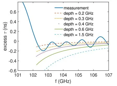
Figure 8. Comparison between the measured perturbation signal to WKB signals including the valley density perturbation with varying depth values.

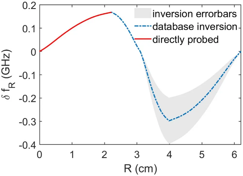
Figure 9. Complete perturbation in the frequency cut-off profile,formed by a directly probed first quarter that is reflected to complete the bump and valley perturbations.

It is clear from observing figure 10 that the new reconstruction scheme for the blind area describes much better the perturbation and eliminates a reminiscent tail of lower density.

As a first approach at this problem,this contribution aims at demonstrating the feasibility of the reconstruction of blind areas using the database of WKB signals of time-of-flight and to show the potential improvements it makes in the reconstructed profiles once applied systematically.A first approach at describing the accuracy of the database reconstruction of blind areas across the full range of parameters has been empirically laid out in[22].The detailed determination of the inversion error bars is however much more reliant on the available signal-to-noise ratio and perturbation frequency band, the precision of the extracted parameters of cut-off gradient and fce, and the estimation of the perturbation width and shape. Therefore, a detailed consideration of the error-bars due to each of these factors is specific to the available conditions at each application. In this specific application, the width, shape and ∇fcutwere assumed wellknow from the considered hypotheses and the dominant source of error was the noise-level when comparing it to the small additional time-of-flight from the perturbation.

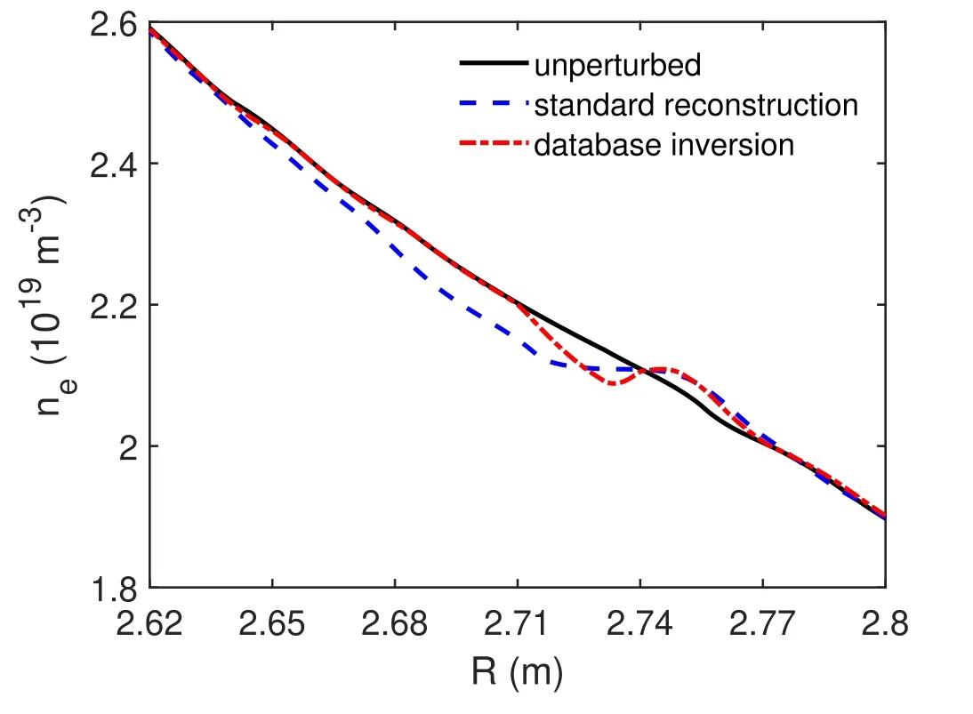
Figure 10.The reconstructed density profiles using the standard reconstruction method on the perturbed and unperturbed measurements versus the new method to reconstruct blind areas introduced in this paper.

4. Final remarks and future prospects

As it was demonstrated, the standard profile reconstruction algorithm adds a significant error in the density profile around and after the blind areas if no special technique is applied around the perturbed region.

This technique was verified to be very accurate in the absence of noise and with precise input parameters when tested on synthetic data. Thus, the final reconstruction precision is expected to come mostly from the available signal-tonoise ratio and the accuracy of the estimated parameters of width, shape, ∇fcutand fcehave been determined, which varies significantly for each application. A detailed consideration of the resulting error bars propagating from the assumptions of the valley shape, width and cut-off gradient will be the focus of future publications where the use of an ultra-fast sweeping rate [27] and the technique to stack multiple sweeps [5] is expected to improve the extracted perturbation signal.

Even though the main physical characteristics of the blind regions have been well described by the 1D simulations[22],additional 2D and 3D simulations[28]will be necessary to verify any additional geometrical aspects. After all, the probing beam area and shape, plus the shape of the perturbations, make in conjunction a system too complex to be completely described in one-dimension as considered here.These aspects influence the amplitude signal across the perturbation bandwidth and the appearance and dynamics of scattering and resonances. Understanding these effects leads to a better extraction of all parameters which is expected to make the database inversion technique more accurate. The research on geometrical aspects will also intersect with the investigation of improved initialization techniques that also observe the time-of-flight and amplitude evolution in the presence of perturbations.

Acknowledgments

This work has been carried out with the support of the Brazilian National Council for Scientific and Technological Development (CNPq) under the Science Without Borders programme,within the framework of the French Federation for Magnetic Fusion Studies (FR-FCM) and of the EUROfusion consortium with funding from the Euratom research and training programme 2014–2018 and 2019–2020 under grant agreement No. 633 053, and also been part-funded by the RCUK Energy Programme [grant number EP/P012450/1].The views and opinions expressed herein do not necessarily reflect those of the European Commission.

ORCID iDs

Rennan B MORALES https://orcid.org/0000-0003-0667-3356

Stéphane HEURAUX https://orcid.org/0000-0001-7035-4574