A number theoretic method for high order correlation functions of the Ulam map

ZHOU Xing-Wang

(College of Mathematics, Sichuan University, Chengdu 610064, China)

Abstract: In this paper, a number theoretic method is introduced to calculate the high order correlation functions of the Ulam map. In this method, the calculation is firstly transformed into solving a class of exponential Diophantine equations with variable coefficients. Then these equations are simplified to the Diophantine equations with strictly monotonic exponentials. Finally, the equations are solved by means of a order reduction method.As an application, the first five order correlation functions of the Ulam map are calculated.

Keywords: Ulam map; Correlation function; Exponential Diophantine equation

1 Introduction

In statistical description of a dynamical system involving internal or external noises, correlation functions of the system play a key role. For a linear system involving Gaussian noises only, the first two correlation functions are sufficient to describe the system. On the other hand, for a nonlinear system or a linear system driven by non-Gaussian noises, all correlation functions of the system are indispensible.

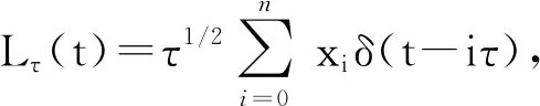
Generally, a correlation function of a dynamical system can be calculated ( in exact or asymptotic manner ) in terms of the correlation functions of the involved noise. For instance, the correlation functions of a dynamical system of Langevin type[1-3], which is a deterministic analogy of Langevin dynamical system, can be calculated by using the correlation functions of the Langevin like noise. And the correlation functions of the Langevin like noise are further calculated by using the correlation functions of the chaotic map. Here the Langevin like noise is a time-scaled impulsive series iteratively generated by a chaotic map, such as tent map, Bernoulli shift map, Ulam map, Tchebyscheff map, etc.

Given an ergodic chaotic map T, a phase space X, and an invariant measure μ of T, the k-th correlation functions of T is defined by

(1)

TN(x)=cos(Narccosx)

(2)

Meanwhile, also by the method of Beck[4], Hilgers and Beck[6]discussed some properties of the correlation functions of the Tchebyscheff maps in 2001.

In this paper,we introduce a number theoretic method to calculate the high order correlation functions of Ulam map. In this method, the calculation is transformed into solving a class of Diophantine equations with monotonic exponentials in a hierarchical manner. As an application, the first five order correlation functions of the Ulam map are calculated.

2 Preliminaries

Following Refs. [4-5], we set x0=cosπu, where u is a random variable obeying the uniform distribution on [0,1]. The iterates of Ulam map can be rewritten into

xn=cosπ2nu

(3)

Inserting (3) and the invariant measure[8]

into (1),the k-th correlation function of Ulam map reads

(4)

For instance, The first four order correlation functions of the logistic map are[5]

E(xn)=0

(5)

E(xn1xn2)=δ(n1,n2)/2

(6)

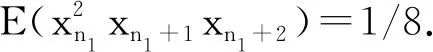
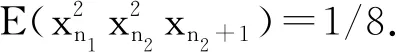
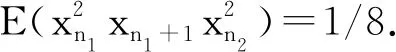
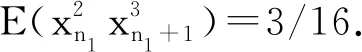
E(xn1xn2xn3)=

(7)

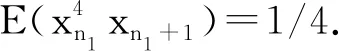
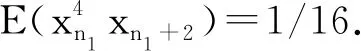
E(xn1xn2xn3xn4)=

ni4)-3δ(n1,n2)δ(n1,n3)δ(n1,n4)/8

(8)

(9)

for given tuple (λ1,λ2,…,λk). In such a way, the calculation fo (4) can be transformed into solving Eq.(9), which can be handled in a straightforward manner.

Due to the symmetry of correlation function (4), we need only to consider the following equation with monotonic exponentials:

(10)

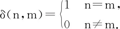
Definition2.1For given (λ1,λ2,…,λk), x1=n1,x2=n2,…,xk=nk, denoted by (n1,n2,…,nk), is called a solution of Eq.(10) if

α1=1, M1=#{xj|xj=x1,j=1,2,…,k},

αi=αi-1+Mi-1,i=2,3,…,s,

Mi=#{xj|xj=xαi,j=αi,αi+1,…,k},

i=2,3,…,s,

yi=xαi,i=1,2,…,s,

where # denotes the number of elements in a finite set, Miis called the multiplicity of xαi.

Definition2.3[9]Let n>0 be a positive integer. We define

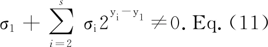
After eliminating the repetition of the exponentials by using Definition 2.2, Eq.(10) reduces to the equation with strictly monotonic exponentials:

(11)

where

(12)

Lemma2.4For every σi,i=1,2,…,s, we have:

(i) σiruns over the finite set

I(Mi)={±Mi,±(Mi-2),…,±(Mi-

2mi),…}

(13)

(ii) σishares the parity with Miwhenever σi≠0;

(iii) 0∈I(Mi) if and only if 2|Mi,where miis the number of the summands λαi+j=-1 in (12).

ProofSuppose that there are mi,mi=0,1,…,Misummands λαi+j=-1 and thus Mi-misummands λαi+j=1 in (12). We have

σi=(Mi-mi)-mi=Mi-2mi

(14)

(i) and (ii) follow.Furthermore, from (14) we get that 0∈I(Mi) if and only if mi=Mi/2 is an integer, which indicates 2|Mi. This ends the proof.

Corollary2.5When 2⫮M1, Eq.(11) has no solution.

ProofEq.(11) is equivalent to

(15)

Theorem2.6When M1=2,Mi=1,i=2,3,…,s, Eq.(11) has only one solution (n,n+1,…,n+s-1) for σ2=σ3=…=σs-1=σ1/2,σs=-σ1/2.

ProofWhen M1=2,Mi=1,i=2,3,…,s, we have σ1∈{0,±2},σi∈{±1},i=2,3,…,s from Lemma 2.4. If σ1=0, then we know that Eq.(11) has no solution from Corollary 2.5.

When σ1=±2, We rewritte Eq.(11) into

(16)

(17)

where q1+σ2∈{0,±2}. Also from Corollary 2.5, we know that Eq.(17) has solution only for y3=y2+1 and q1+σ2=±2. That is to say, q1=σ2. Thus Eq.(17) turns to

which shares the structure with Eq.(16) with s-1 variables, where q2=(q1+σ2)/2, say, q1=σ2=q2.

Repeating above discussion, we finally realize that Eq. (11) has solution if and only if q1=σ2=…=σs-1=qs-1, yi+1=yi+1,i=1,2,…,s-2 and

qs-12ys-1+1+σs2ys=0,ys-1+1≤ys. It istrivial to know that the above equation has solution ys=ys-1+1 for σs=-qs-1. Let y1=n. The proof is complete.

3 The solutions of Eq.(11) with 3 variables

Theorem3.1When s=1, Eq.(11) has only one solution y1=n for σ1=0.

Lemma3.2The Diophantine equation

q1+q22x=0,ord2qi=0,i=1,2

has only one solution x=0 for q1+q2=0.

Theorem3.3When s=2, Eq.(11) has the following three solutions:

(i) (n1,n2) for (0,0);

(ii) (n,n+l) for (2lq1,-q1);

(iii) (n,n+r) for (2l1q1,2l2q2), where ord2(q1q2)=0,q1+q2=0, and r=l2-l1≥1.

ProofWhen s=2, Eq.(11) shrinks to

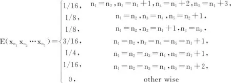
σ12y1+σ22y2=0,y1

(18)

From Corollary 2.5, Eq.(18) has no solutionwhen ord2(σ1σ2)=0. Then the solution of Eq. (18) can be divided into three cases.

Case1. σ1=0 or σ2=0. The solution (i) comes from Theorem 3.1.

Case2.2|σ1,2⫮σ2. After setting σ1=2lq1,ord2q1=0, Eq.(18) can be rewritten into

q1+σ22y2-y1-l=0,y1

(ii) follows from Lemma 3.2.

Case3.2|σi,i=1,2. By setting σi=2liqi,ord2(q1q2)=0, Eq.(18) can be rewritten into q12y1+l1+q22y2+l2=0,y1

q1+q22y2-y1+l2-l1=0,y1

(19)

Then， by taking the transformation x=y2-y1+l2-l1, the only solution y2=y1+l1-l2for q1+q2=0 follows from Lemma 3.2. Furthermore, considering the condition y1

When s=3, Eq.(11) is

σ12y1+σ22y2+σ32y3=0,y1

(20)

Obviously,when at least one σi=0,i=1,2,3, Eq.(20) shrinks to Eq.(18), which has been solved in Theorem 3.3. Especially, Eq.(20) has solutions (n1,n2,n3) for (0,0,0).

Since Eq.(20) has no solution when 2⫮σ1, we assume 2|σ1in what follows.

Lemma3.4Suppose that ord2(qi)=0,i=1,2,3. Then the following Diophantine equation

q1+q22x+q32y=0,x,y∈Z

(21)

has three solutions:

(i) (0,l1) for p1+q3=0;

(ii) (l3,0) for q2+p3=0;

(iii) (-l2,-l2) for q1+p2=0,

where q1+q2=2l1p1, q2+q3=2l2p2, q3+q1=2l3p3,ord2(pi)=0,i=1,2,3.

ProofWhen x=0 or y=0, Eq.(21) has been considered in Lemma 3.2. We get (i) and (ii).

When xy≠0, after setting u=min{x,y}≠0 and rewriting Eq.(21) into

q12-u+q22x-u+q32y-u=0,x-u≥0,y-u≥0

(22)

we divide the proof into the following two cases.

Case1.x≠y. We have x-u=0,y-u>0 or y-u=0,x-u>0. Without lose of generality, we consider the former. In this case Eq.(21) is

q2+q12-u+q32y-u=0,y-u>0

(23)

If u>0, then 2|q32y-uand q2+q12-uis not an integer, which means that Eq.(21) has no solution. If u<0, since 2⫮q2， 2|(q12-u+q32y-u), Eq.(21) has no solution as well.

Case2.x=y=u. In this case, Eq.(21) turns to

q1+(q2+q3)2x=0,x∈Z

(24)

which is

q1+p22x+l2=0,x∈Z

(25)

(iii) follows from Lemma 3.2. The proof is end.

Theorem3.5Suppose that σ1=2rq1,ord2(q1)=0 and ord2(σ2σ3)=0. Then Eq.(20) has only one solution (n,n+r,n+r+l1) for σ3+p1=0, where q1+σ2=2l1p1,ord2(p1)=0.

ProofSubstituting σ1=2rq1into Eq.(20) yields that

q12y1+r+σ22y2+σ32y3=0,y1

(26)

which is

q1+σ22y2-y1-r+σ32y3-y1-r=0,y1

Taking the transformation

x=y2-y1-r∈Z,y=y3-y1-r∈Z

(27)

Eq.(26) recovers Eq.(21) with x0 for σ3+p1=0. The proof is ended by taking the inverse transformation of (27).

Theorem3.6Suppose that σi=2riqi,ord2(qi)=0,i=1,2 and ord2(σ3)=0. Then Eq. (20) has three solutions:

(i) (n,n+r1-r2,n+r1+l1) for r1>r2,q3+p1=0;

(ii) (n,n+r1-(r2-l3),n+r1) for r1>r2-l3>0,q2+p3=0;

(iii) (n,n+r1-r2-l2,y2+r2) for r1>r2+l2,q1+p2=0,

where q1+q2=2l1p1, q2+q3=2l2p2, q3+q1=2l3p3,ord2(pi)=0,i=1,2,3.

ProofSubstituting σi=2riqi,i=1,2 into Eq. (20) yields

q12y1+r1+q22y2+r2+σ32y3=0，y1

(28)

which is

q1+q22y2-y1+r2-r1+σ32y3-y1-r1=0，

y1

Taking the transformation

x=y2+r2-y1-r1∈Z,y=y3-y1-r1∈Z

(29)

Eq. (28) recover Eq.(21). The needed results follow immediately from Lemma 3.4 by checking the monotonicity of the exponentials in Eq. (28).

Theorem3.7Suppose that σi=2riqi,ord2(qi)=0,i=1,3, and ord2(σ2)=0. Then Eq. (20) has solution (n,n+r1,n+r1+l1-r3) for l1>r3,q3+p1=0, where q1+q2=2l1p1,ord2(p1)=0.

ProofAfter substituting σi=2riqi,i=1,3 into Eq. (20), we get

q12y1+r1+σ22y2+q32y3+r3=0，

y1

(30)

which is

q1+σ22y2-y1-r1+q32y3+r3-y1-r1=0,

y1

By taking the transformation

x=y2-y1-r1∈Z,y=y3+r3-y1-r1∈Z

(31)

Eq. (30) recovers Eq. (21). The desired results follow from Lemma 3.4 by taking the condition x

Theorem3.8Suppose that σi=2riqi,ord2(qi)=0,i=1,2,3. Then Eq. (20) has five solutions:

(i) (n,n+r1-r2,n+r1+l1-r3) for r1>r2,

l1>r3-r2,q3=-p1;

(ii) (n,n+r1-r3,n+r1+l1-r3) for r1>

r3=r2,q3=-p1;

(iii) (n,n+r1-r2,n+r1+l1-r3) for r1>

r2>r3,q3=-p1;

(iv) (n,n+r1-(r2-l3),n+r1-r3) for r1>r2-l3>r3,q2=-p3;

(v) (n,n+r1-(r2+l2),y2+r2-r3) for r1>r2+l2,r2>r3,q1=-p2,

where q1+q2=2l1p1, q2+q3=2l2p2, q3+q1=2l3p3, and ord2(pi)=0,i=1,2,3.

ProofAfter substituting σi=2riqi,i=1,2,3 into Eq. (20), we arrive at

q12y1+r1+q22y2+r2+q32y3+r3=0,y1

(32)

Let r0=min{r1,r2,r3}. The proof can be divided into the following three cases.

Case1.r0=r1. Let u2=r2-r1≥0,u3=

r3-r1≥0. Eq. (32) turns to

q1+q22y2-y1+u2+q32y3-y1+u3=0,

0

(33)

Since 2⫮q1, We know from Corollary 2.5 that Eq. (33) has no solution.

Case2.r0=r2. Let u1=r1-r2≥0,u3=

r3-r2≥0. Eq. (32) turns to

q12y1+u1+q22y2+q32y3+u3=0,y1

(34)

which recovers Eq. (30). Then (i) follows from Theorem 3.7.

Case3.r0=r3. Let u1=r1-r3≥0,u2=

r2-r3≥0. Eq. (32) turns to

q12y1+u1+q22y2+u2+q32y3=0,y1

(35)

If u1=0, then we know from Corollary 2.5 that Eq. (35) has no solution. If u1>0,u2=0, then Eq. (35) turns to

q12y1+u1+q22y2+q32y3=0,y1

(36)

which recovers Eq. (26). (ii) follows from Theorem 3.5. If u1>0,u2>0, then Eq. (32) turns to

q12y1+u1+q22y2+u2+q32y3=0,y1

(37)

which recovers Eq. (28). (iii)～(v) follow from Theorem 3.6. The proof is end.

4 The first five order correlation functions of the Ulam map

In this section, as an application of the method, we calculate the first five order correlation functions of Ulam map by solving Eq.(9) and Eq.(11).

When k=1, Eq.(9) has no solution,

E(xn1)=0.

When k=4, after excluding the cases of no solution by Corollary 2.5, Eq. (9) turns to σ12y1=0 with σ1=0,±2,±4, or Eq. (18) with σ1=0,±2,σ2=0,±2, or Eq. (20) with σ1=0,±2,σ2=±1,σ3=±1.

Case2.M1=M2=2,M3=1. In this case, we have σ1=0,±2,σ2=0,±2,σ3=±1. When σ1=σ2=0, we know Eq. (11) has no solution from Corollary 2.5.

When σ1=±2,σ2=0,σ3=±1, Eq. (11) also shrinks to Eq. (18). Since the only possible solution (n1,n2,n1+1) violates the monotonicity of the exponentials, Eq. (9) has no solution.

When σ1=±2,σ2=±2,σ3=±1, Eq. (11) turns to Eq. (20). By Theorem 3.6, we get r1=r2=1,q1=±1,q2=±1,q3=±1. Since r1=r2=1violates the conditions r1>r2,r1>r2-l3>0, and r1>r2+l2in Theorem 3.6, Eq. (9) has no solution.

Case3.M1=M3=2,M2=1. In this case, we get σ1=0,±2,σ2=±1,σ3=0,±2. When σ1=0, we know Eq. (11) has no solution from Corollary 2.5, since 2⫮σ2.

When σ1=±2,σ2=±1,σ3=±2, Eq. (11) turns to Eq. (20). By Theorem 3.7, we have r1=r3=1,q1=±1,q2=±1,q3=±1, which yields that q1+q2=0,±2. It is trivial to get that Eq. (11) has no solution when q1+q2=0. In the case of q1+q2=±2, we get l1=r3=1, which indicates the condition l1>r3in Theorem 3.7 can't be fulfilled. Thus Eq. (11) has no solution.

Finally, we conclude that

(38)

5 Conclusions

This paper aims at the calculation of high order correlation functions of the Ulam map. We introduce a number theoretic method including definitions, lemmas, and theorems, and transform the calculation into solving a class of Diophantine equations with strictly monotonic exponentials. Then, by solving the exponential Diophantine equations with variables less than 4, we get the first five order correlation functions of the Ulam map. Compared with the graph theoretic method, our method is straightforward and fruitful.

A zero-centered noise is called to be dynamical asymmetric[10-12], if some of its odd order correlation functions are non-vanishing other than the first order correlation function. Remarkably, a dynamical asymmetric noise alone can induce a directed current in a spatial symmetric periodic structure. Interestingly, it had been shown that, for instance in Refs. [13-14], a Langevin type noise generated by the logistic map could induce a negative current in a spatial symmetric periodic potential. The coincidence of the sign between the current and the odd order correlation functions of the logistic map mentioned us that there is intrinsic correlation between the direction of the current and the sign of the odd order correlation functions of the chaotic map.