Differentially Private Real-Time Streaming Data Publication Based on Sliding Window Under Exponential Decay
Lan Sun, Chen Ge, Xin Huang, Yingjie Wu, and Yan Gao
Abstract: Continuous response of range query on steaming data provides useful information for many practical applications as well as the risk of privacy disclosure. The existing research on differential privacy streaming data publication mostly pay close attention to boosting query accuracy, but pay less attention to query efficiency, and ignore the effect of timeliness on data weight. In this paper, we propose an effective algorithm of differential privacy streaming data publication under exponential decay mode. Firstly, by introducing the Fenwick tree to divide and reorganize data items in the stream, we achieve a constant time complexity for inserting a new item and getting the prefix sum. Meanwhile, we achieve time complicity linear to the number of data item for building a tree. After that, we use the advantage of matrix mechanism to deal with relevant queries and reduce the global sensitivity. In addition, we choose proper diagonal matrix further improve the range query accuracy. Finally, considering about exponential decay, every data item is weighted by the decay factor. By putting the Fenwick tree and matrix optimization together, we present complete algorithm for differentiate private real-time streaming data publication. The experiment is designed to compare the algorithm in this paper with similar algorithms for streaming data release in exponential decay. Experimental results show that the algorithm in this paper effectively improve the query efficiency while ensuring the quality of the query.
Keywords: Differential privacy, streaming data publication, exponential decay, matrix mechanism, sliding window.
1 Introduction
Currently, the rapid development of big data and the Internet of things (IoT) makes data easier to be collected, and leads to a serious concern about information security [Yang and Soboroff (2015)]. Specially, many applications require continuous statistical release of streaming data, such as real-time statistics of the sales amount on shopping sites,real-time statistics of high frequency phrases for search engines. In these applications, the release data is the accumulated value of streaming data in a certain sense. Statistical publication of streaming data not only brings information to people's life, but also brings the risk of privacy disclosure [Fung, Wang, Chen et al. (2010)]. Differential privacy[Dwork (2006); Zhou, Li and Tao (2009); Xiong, Zhu and Wang (2014); Zhang and Meng (2014)] is recognized as a robust privacy protection model. In view of the privacy protection of streaming data publication, there are many related studies based on differential privacy model. There is a lot of related research [Dwork, Naor, Pitassi et al.(2010); Chan, Shi and Song (2010); Cao, Xiao, Ghinita et al. (2013); Zhang and Meng(2016); Bolot, Fawaz, Muthukrishnan et al. (2013)] for privacy protection of streaming data release is based on differential privacy model.
Dwork et al. [Dwork, Naor, Pitassi et al. (2010)] put forward a study of differential privacy under continual observation. It continuously releases the count value of single stream data from start to current time by piece-wise counting. Chan et al. [Chan, Shi and Song (2010)]improved the query accuracy and algorithm efficiency by binary tree. Zhang et al. [Zhang and Meng (2016)] realized the publication of count values in each sliding window with partitioning-based method.
There are two problems in existing correlation studies: 1. All of the above studies assume that the data items at all times are of the same importance. But in practical applications, it tends to pay more attention to the statistical release of recent data and low attention to historical data because the statistical monitoring of recent events has a stronger relevance to its purpose. To solve this problem, a usually method is to make the data item with weight which is inversely proportional to the distance from the data to the current time. Under exponential decay mode, Cao et al. [Cao, Xiao, Ghinita et al. (2013)] proposed differential privacy streaming data publishing algorithm with interval tree structure which is failure to make full use of the correlation between queries in continuous statistical publishing to further improve the accuracy of data release. 2. Authors in Dwork et al. [Dwork, Naor,Pitassi et al. (2010); Chan, Shi and Song (2010); Cao, Xiao, Ghinita et al. (2013); Zhang and Meng (2016); Bolot, Fawaz, Muthukrishnan et al. (2013)] mainly focused on how to improve the query precision of streaming data. However, here is a higher demand for the query efficiency of data release in many practical applications.
In this paper, we present a differential privacy real-time release algorithm for streaming data in exponential decay mode. This algorithm effectively improves the query efficiency on the premise of guaranteeing the quality of the streaming data.
The main works of this paper are as follows:
(1) Point at continuous statistical release of streaming data under exponential decay mode,we propose an algorithm to improve efficiency of range query with Fenwick tree.
(2) Furthermore, matrix mechanism is used to explore the relevance between queries.Algorithms for strategy matrix construction and diagonal matrix construction are proposed according to the characteristics of the load matrix under exponential decay mode. The matrix optimization method is used to further improve the query accuracy and efficiency.(3) We present complete algorithm of streaming data range query response under exponential decay. Experimental results show that the algorithm is effective and feasible.The organizational structure of the rest of this paper is as follows: The second section gives a brief introduction of the relevant concepts. The third section describes our approach and provides theoretical analysis. Section 3.1 proposes a fast range query algorithm based on Fenwick tree. How to introduce the matrix mechanism to improve the release accuracy is explained in Section 3.2. Experimental results and analyses are presented in Section 4, and Section 5 is the conclusion.
2 Background
2.1 Differential privacy
Differential privacy [Dwork (2006)] has gradually emerged as the standard notion of privacy in data analysis. Informally, an algorithm is differential private if it is insensitive to small changes in the input. The formal definition of “small changes” is as follows:
Definition 1(Neighboring data sets): Given two data setsDandD’, if they are differing on at most one element:

Then we call them a pair of neighboring data sets.
Definition 2(ε-differential privacy): Algorithm A isε-differential private if for any neighboring data setsDandD’, and any subset of outputs S⊆Range(A), the following holds:

where the probability is taken over the randomness of theA. The smaller theε, the stronger the private protection is.
2.2 Range Query in Sliding Window under Exponential Decay
Definition 3(Sliding window): Arrange items in a streaming data according to their time stamp. The sliding window, with a fixed lengthW, always keeps the newestWth items,while discarding old ones.
Definition 4(Range query in sliding window): Range query is to accumulate all items in a continuous interval in sliding window. Formally, for a data streamS ={D1, D2, ..., Dn}, and the current time ist. The answer of the range query

Definition 5(Range query under exponential decay): Based on definition 4, we add the weight coefficientto each data item, whereis called the decay factor which is fixed beforehand, the variablexrepresents the distance between the item’s time stamp andt. The above formula is adjusted to:

Exponential decay associates longer items with smaller impact on final result.
2.3 Matrix mechanism
Given a workload of linear range queries, the matrix mechanism [Li, Hay, Rastogi et al.(2010); Yuan, Zhang, Winslett et al. (2012)] uses an alternative set of queries, named the strategy, which are answered privately by a standard mechanism. Answers to the workload are then derived from the strategy queries, which bringing a higher accuracy.
Definition 6(Matrix mechanism): Decompose the workload matrixWinto two matricesBandL. We callLthe strategy matrix, which actually making a basis transformation on original data. Then noise is added to the result of transformation, and the disturbing result is converted to the final query result through matrixB. The formula form is as follows:

3 Real-time private streaming data publication under exponential decay
3.1 Real-time range query based on Fenwick tree
As proposed in Chan et al. [Chan, Shi and Song (2010)], one can use interval tree as the data structure to arrange streaming data in the sliding window, which improves the time efficiency of data release. Specifically, full binary tree architecture was used in Chan et al.[Chan, Shi and Song (2010)], and its structure is shown in Fig. 1. Assume the size of sliding window isW, andtrepresents the current moment. As shown in Fig. 1, there are two binary trees that each has its part included in sliding window. Gray nodes were slid out of the window and will never be concerned again in later process, while striped ones are about to be included. Once first node of the new tree has been included, the whole binary tree will be built beforehand. Nodes in the new tree will be activated one after another in pace with their sliding into the window.
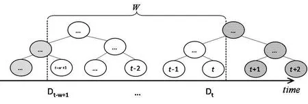
Figure 1: Building interval tree under sliding window
Using the full binary tree, we can answer any range query in the sliding window. However,as Fig. 2 suggested, all of the right sons (gray nodes) in the tree are unnecessary for this job,because we can obtain their value by their father nodes. By removing them, the number of remain nodes is equal to the size of sliding window, i.e.W. And we can still add every emerging data item in a constant time. After this simplification, the remained structure is called Fenwick tree [Fenwick (1994)].
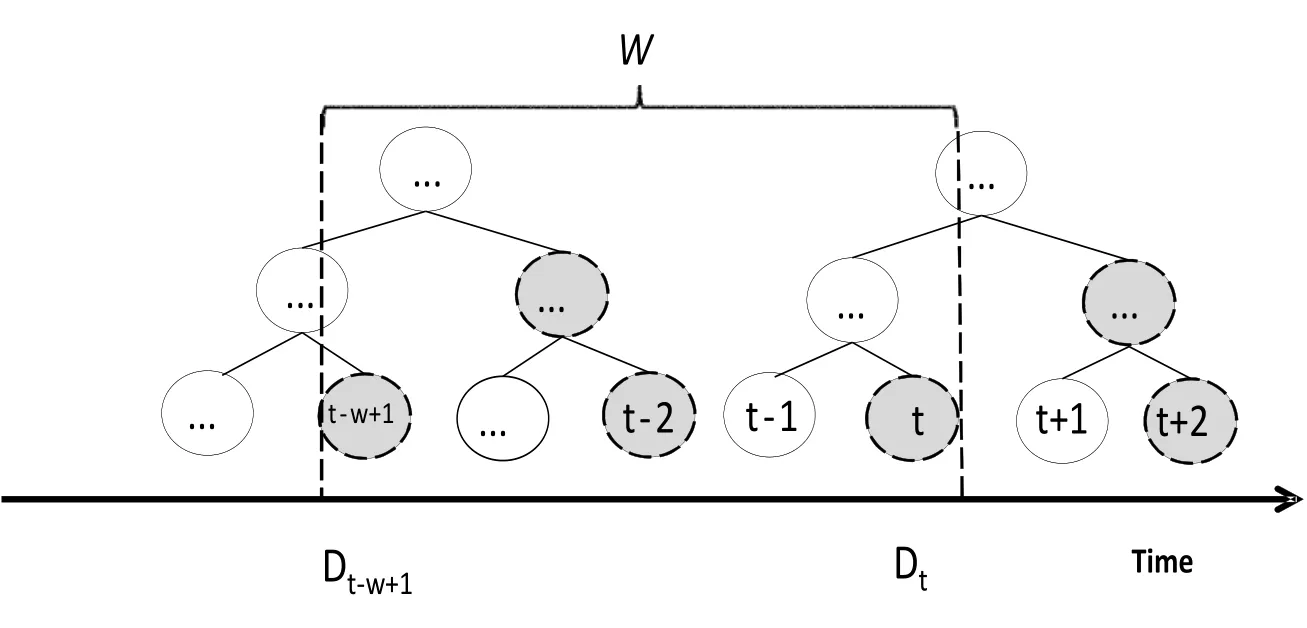
Figure 2: The gray nodes are redundant
Fenwick tree is such a data structure that supports query and modify operation with aO(log2(N)) time complexity. For a givenr, the prefix sum in range [1,r] can be figure out quickly. We useSum(r) to represent the prefix sum, i.e.Sum(r)=D1+D2+...+Dr(we neglect the exponential decay temporarily).
In the calculating process, Fenwick tree has generated intermediate variablesSi(i∈[1,r]),given by the following formula:

Djis the j-th data item, andlowbit(x) means the lowest “1” in the binary form ofx. For example, when x=12, we have (12)10=(1100)2. The lowest “1” is in the third position, solowbit(12)=(0100)2=(4)10. We can getlowbit(x) easily by bitwise operation:lowbit(x)=x& (-x). Fenwick tree then use these intermediate variablesSito get the prefix sum:

When considering about exponential decay, every data item should be weighted by the decay factorpx. So the prefix sum becomes:

Correspondingly, formula (8) and formula (9) are also adjusted to formula (11) and formula (12) as follows:

Fig. 3 shows the structure of Fenwick tree under exponential decay.

Figure 3: Fenwick tree under exponential decay
In Fig. 3, the size of sliding window, i.e.W, is 5, so we choose the tree’s height to be 3.Nodes which have already slid out of the window will never be used again, so we can recycle them to save memory. And once after the latest node of old tree has been processed,the next data item will cause the building process of a new tree with preset height.
Then we give the detail about how the Fenwick tree works:
Firstly, we number activated nodes according to their time stamp. Then the white nodes in Fig. 4 form two Fenwick trees. One contains nodes ①~④, while nodes ⑤~⑦ stored in another. The value of node ① is the data item at timet1, ②’s value is the sum oft1andt2,and ④ is sum of [t1,t4]. (When considering about exponential decay, all the value mentioned above should be associated with their decay weight. For simplicity, we omit the statement about it. You can see Fig. 3 and algorithm 1 to get a better understanding).
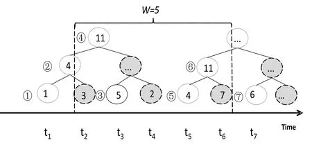
Figure 4: Details about Fenwick tree
Briefly, father’s value is the sum of all its sons (We call nodeyis the father of nodex, ifx +lowbit(x)= y). And we just need one add operation for each node, because its father is unique. Let us take node ④ for example: It is only father of nodes ② and ③. So after calculating node ②, we can immediately add it to node ④, withO(1) time cost. Therefore,we achieve time complicity linear to the number of data item for building a tree.
Then we can use such a tree structure to get the prefix sum. For example,Sum(1)=t1is the value stored in node ①,Sum(2)=t1+t2is the value in node ②, andSum(3)=t1+t2+t3is the sum of nodes ② and ③. As forSum(5)=t1+...+t5, because it is split into two trees, we need to sum up nodes ④ and ⑤. We can further simplify this process. For example, since we has already get the prefixSum(6)=⑥+④, we can getSum(7)=⑦+⑥+④ by sum upSum(6) and node ⑦. By this way, we achieveO(1)time complicity for inserting a single new node.
WhenWwas given, the tree’s height is then determined, writtenH. Based on formula (9),the global sensitivity is alsoH. Therefore, by adding Laplace noise with scaleH/εto each node in the tree, our algorithm satisfiesε-differential privacy.
In summary, the algorithm for inserting new data item into Fenwick tree is described in algorithm 1:
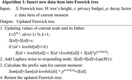
3.2 Accuracy optimization using matrix mechanism
To answer a range query, we may need to combine some nodes’ values generated in last section. For example, in Fig. 4, we have to answer the range query [2, 5] by [1, 4]+[4,5]-[1, 2].It causes the accumulation of noise, and then the loss of accuracy. In Section 3.1, we have generated intermediate variablesSiby Fenwick tree. This process can be written as a form of a matrix timing a vector. When the size of tree is 7, the matrix and vector is as follows:

WhereLis the strategy matrix,Dis the original data set, andSis a vector combined by all intermediate variablesSi. That is to say, we transform the original data set into the intermediate variables vector, perturb it using Laplace noise, and finally restore it for answering the queries. This process is corresponding to formula (11) and Fig. 3.
Correspondingly, when given a certain Fenwick tree, we can restore it to the prefix sums that we need, using formula (12). We follow the example above, giving the matrix form for this restoring process:

WhereWis the load matrix. In our setting of continual range query response, its form is as follows:

In conclusion, the prefix vector can be written as matrix formWD=BLD, whereW=BL.After changing the tree into a matrix form, our method is actually a specific decomposition strategy of matrix mechanism. The matrix mechanism, in general, is to design an optimal decomposition strategy to decompose the workloadWto improve accuracy. However, we aim to design a sub-optimal decomposing way, whose error is slightly greater than the optimal one. But we can figure out it quickly following Section 3.1’s result. According to Yuan et al. [Yuan, Zhang, Winslett et al. (2012)], the mean square error of our method is:

LetNbe the size of matrix, concluded from formula (8), the number of nonzero elements in each row of reduction matrixBis not greater thanlog2(N), and total number of nonzero elements in B is not larger thanN·log2(N).Since the only possible value of nonzero elements in B is 1, we havetrace(BTB)≤N·log2(N).By formula (2) to formula (7), the global sensitivity ofL, i.e. ΔL, is equal to the tree’s heightH=log2(N). The total error of all N times query isAveraging to each query, the mean error isAccording to Cai et al. [Cai, Wu and Wang (2016)], there exist a diagonal matrixwhich changesand formula (15) is adjusted to:


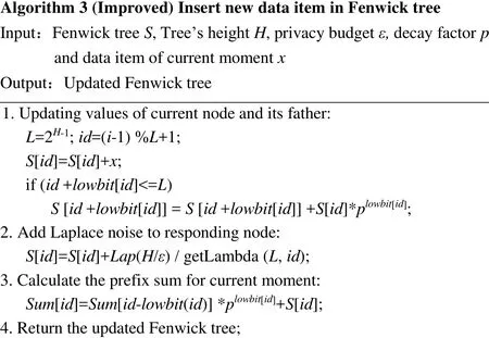
Under our setting of sliding window, since the window’s size is fixed, we can consider this calculation as a preprocessing part. We store the diagonal values beforehand, and invoke them directly during the publishing, avoiding time waste.
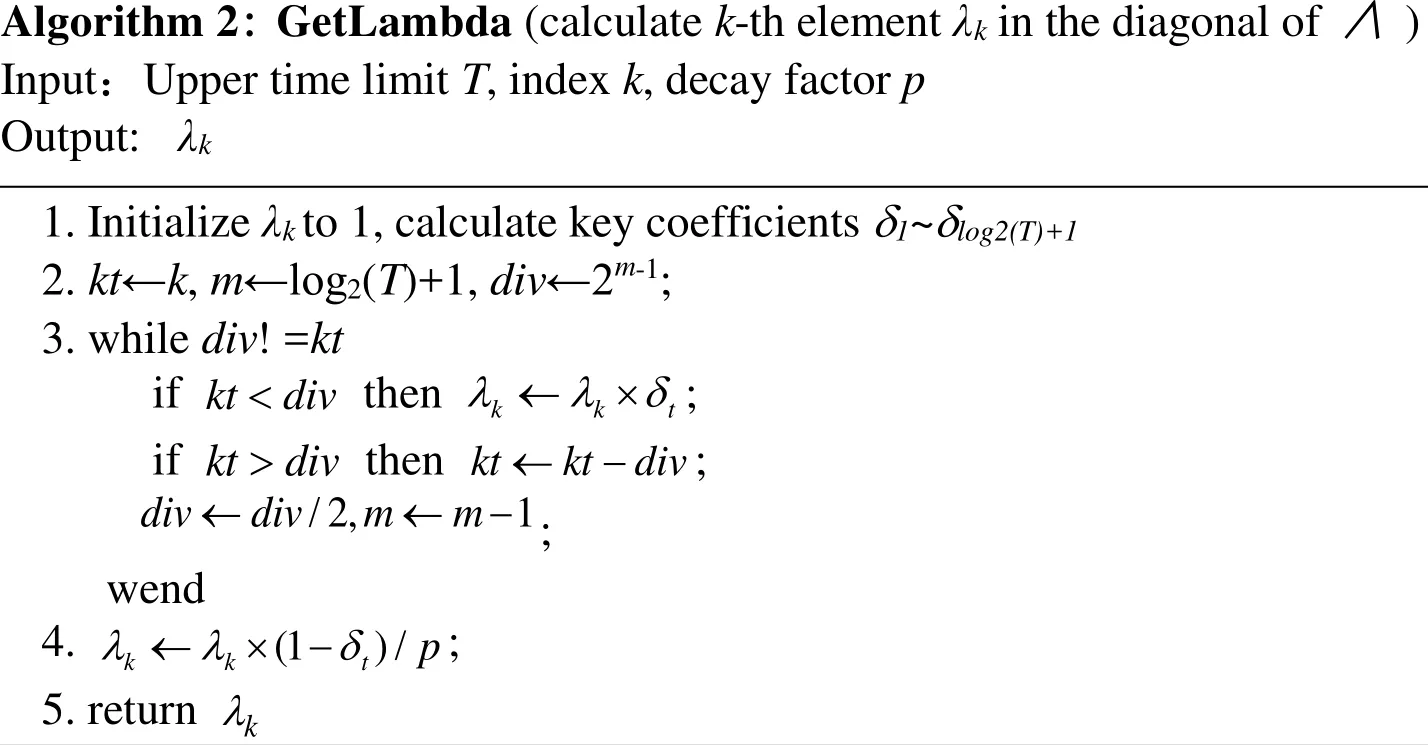
From above analysis, we come to the conclusion that: Though this accuracy optimize method is deduced based on matrix mechanism, there is no need to explicitly calculate the matrices. We can simply adjust algorithm 1 by adding the coefficients from the diagonal matrix. The improved Fenwick tree building algorithm is as follows:
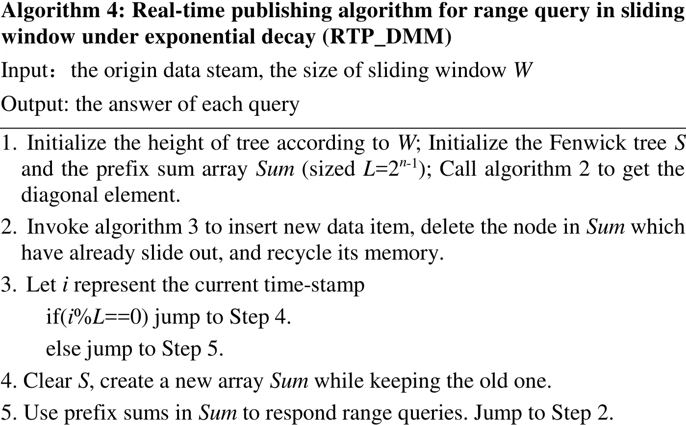
Putting the Fenwick tree and matrix optimization together, we present our complete method in algorithm 4:
4 Experiments
We compare our method, named RTP_DMM, with two similar works in terms of efficiency and accuracy: The EX algorithm proposed in Zhang et al. [Zhang and Meng(2016)] using interval tree; and the LP algorithm proposed by Dwork, which directly calculate the weighted answers and perturb it. We set different privacy budget parameters as 1.0, 0.1 and 0.01. To exclude randomness, each experiment was run 30 times to get the average.
4.1 Data sets and environment
We use the Search Logs and NetTrace in Hay et al. [Hay, Rastogi, Miklau et al. (2010)],along with WorldCup98 in Kellaris et al. [Kellaris, Papadopoulos, Xiao et al. (2014)] as our testing data sets. Search Logs collects the number of searches for the keyword“Obama” from 2004.01 to 2009.08. The NetTrace data sets contain the number of packet requests to a IP segment during a specific period. WorldCup98 records the visits to the World Cup official website during 1998.04 to 1998.07. Their scales are shown in Tab. 1.

Table 1: Scales of data sets
We use the mean square error to measure the query accuracy of the published data, which is shown as follows:

Where|Q|is the number of queries,Dis the original data set,D’is the distributed data set andqrepresents a query.
The experimental environment is: Intel Core i5 4570 3.2 GHz, with 8 GB memory, and we use C++ under Windows 7.
4.2 Comparison and analysis of query efficiency
4.2.1 The effect of different query numbers on efficiency
In this experiment, we set different query numbers at each moment to compare the query efficiency of three algorithms. Because the query efficiency on small data set does not change significantly, the experiment only uses WorldCup98, and the size of the query range is set to 32768. The size of sliding window is fixed to 65536 and the decay factorpis 0.9995.
Different query time of different algorithm is shown in Fig. 5. As the number of queries increases, difference between several algorithms in the running time becomes more obvious. This is because when the number of queries is small, the main influence factor of the efficiency is the cost of model construction. When queries increase, the time spent in the query occupies the dominant position.
Compare with LP and RTP_DMM, the query time of EX increases most rapidly. This is because EX constructs an interval tree to achieve arbitrary range query within the sliding window. Although it reduces the number of nodes involved in a single query, it has to traverse the tree’s height. So the time complexity for a single query isO(log2W), which is log-linear to the size of the sliding window. So the query efficiency is low. RTP_DMM uses the prefix sum to obtain an arbitrary range of query results withinO(1)time. LP also realizes constant time complexity. However, because of the large number of nodes involved in the calculation, its accuracy is terrible. Compared with LP, RTP_DMM needs more complex calculations to reduce the error which brings a larger constant. Therefore, as the number of queries increases, its running time is slightly larger than LP.

Figure 5: Efficiency at different query frequency
4.2.2 The effect of sliding window size on query efficiency
Then we set different sliding window sizes for further comparison. We still only use the WorldCup98 for the same reason. The size is set to 215, 216, ..., 221, respectively. Range size is set to be half of the window’s size, so that this size increases with the window, and the query frequency is set to be once per time.
In Fig. 6, we observe that as the size of the sliding window increases, the RTP_DMM and LP are less affected than EX. The reason behind it is that the sliding window’s size only affects RTP_DMM’s space complexity and preprocessing time. For LP, the query efficiency is independent of the window size. However, as for EX, the time complexity isO(log2W) which is log-linear to window size. So the curve of LP and RTP_DMM are below EX’s. Both LP and RTP_DMM achieveO(1) time complexity, so they have close performance in our experiment.
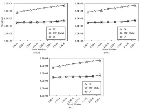
Figure 6: Efficiency under different sliding window sizes (WorldCup98)
4.3 Comparison of query accuracy
We use all three data sets to compare query accuracy between algorithms. Since the scale of Search Logs and NetTrace is small, the length of sliding window is set as the whole data set. As for WorldCup98, Setting the sliding window size to 65536 is suit for further comparison.
4.3.1 Compare accuracy for random range queries
We generate one range query of random size within the sliding window at each moment.Under exponential decay, small decay factor will make the decay speed too fast. So we fixed the decay factorpto 0.9995. The experimental comparison results are shown in Figs. 7-9.
It can be seen from Figs. 7-9 that RTP_DMM reaches significant higher accuracy than LP and EX. This is because RTP_DMM converts range queries into matrix representations,and applies diagonal matrix optimization to improve accuracy. For all three algorithms, the query error increases as the privacy budget decreases. It is because we need larger scale of Laplace noise with smaller privacy budget.

Figure 7: Comparison of query accuracy (Search Logs)

Figure 8: Comparison of query accuracy (NetTrace)

Figure 9: Comparison of query accuracy (WorldCup98)
4.3.2 Accuracy with different decay factors
In this experiment, we compare different decay factors to analyze their influence on the query error. We take the decay factors as 0.9991, 0.9992, ..., 0.9999 respectively.
As the comparison results in Figs. 10-12, the query error is positively correlated with the decay factor, this is because the increase of the decay factor will change the global sensitivity and thus affect the scale of added noise. The EX algorithm calculates the limit of noise scale according to the preset decay factor. Therefore, when the decay factor is close to 1, the average square error caused by the EX algorithm become large. As for the LP algorithm, when the decay factor is small, the weight of the long time nodes tends to be zero which leads to smaller error.
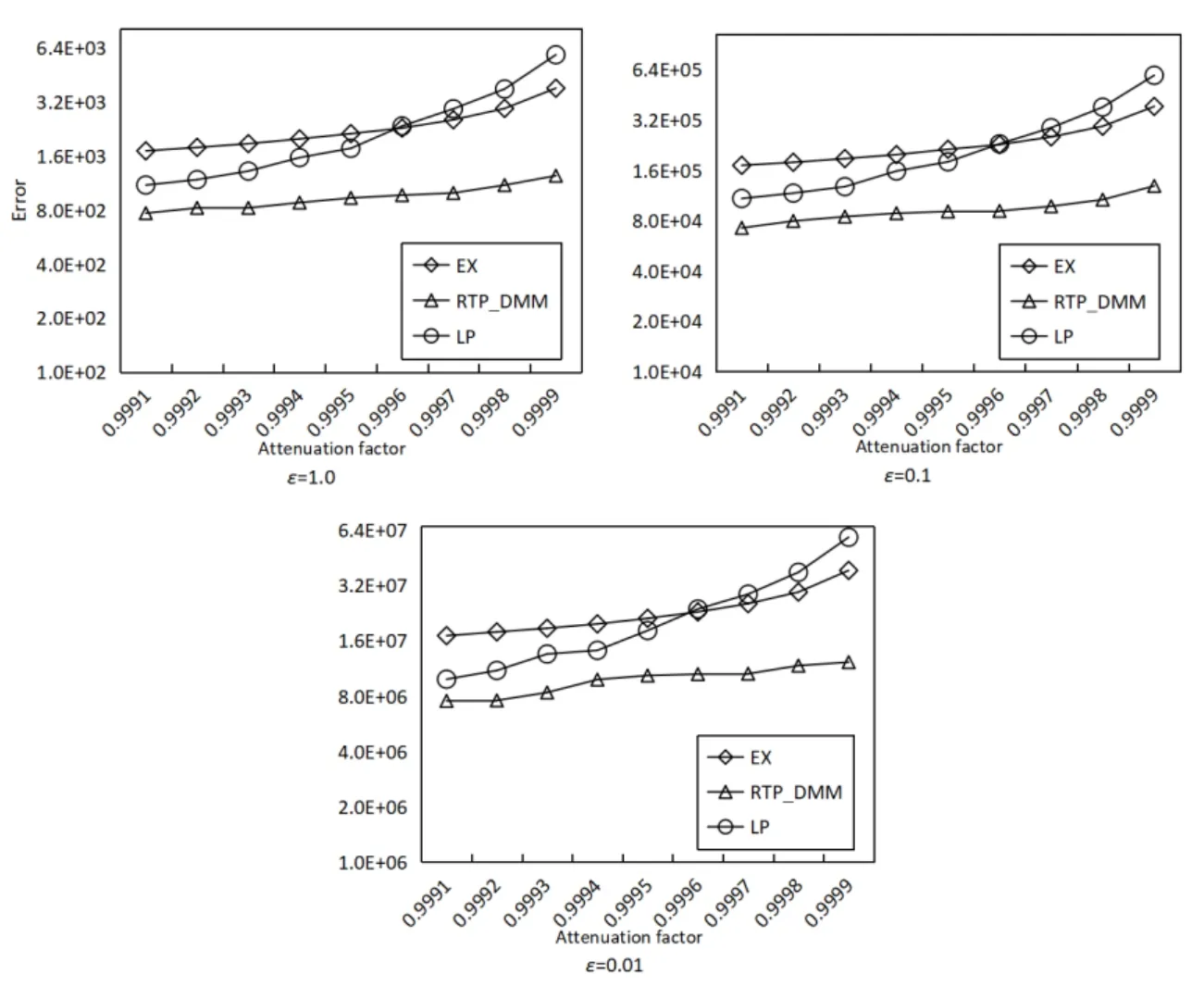
Figure 10: Accuracy with different decay factors (Search Logs)

Figure 11: Accuracy with different decay factors (NetTrace)
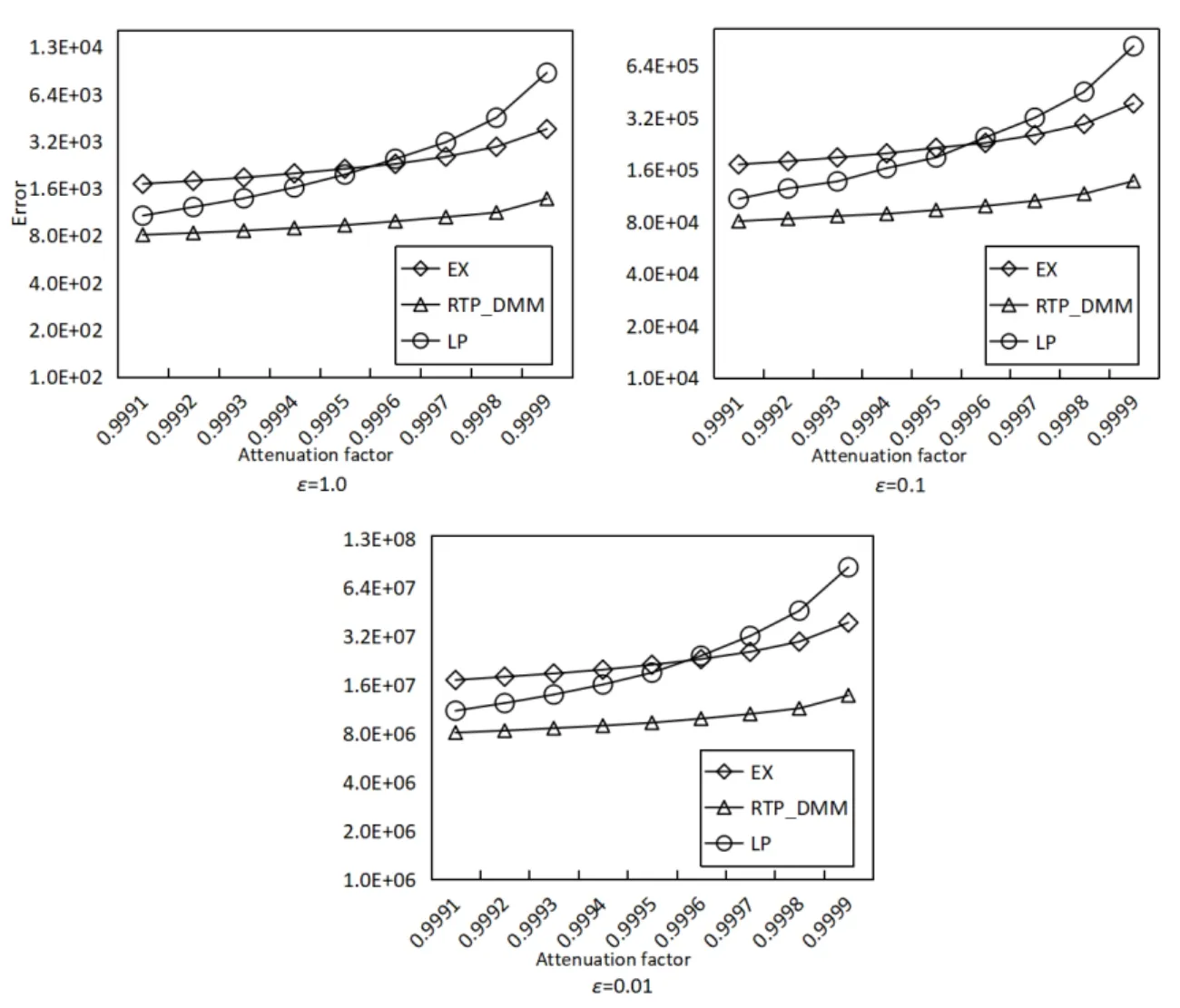
Figure 12: Accuracy with different decay factors (WorldCup98)
Based on the above experiments, it can be concluded that the algorithm RTP_DMM is scalable for different applications with various decay factors and privacy budget. It can reduce query error, and achieve real-time publishing under the sliding window.
5 Conclusion
In this paper, we propose an efficient method for real-time differential privacy streaming data publishing under exponential decay. It answers any range query within the sliding window inO(1) time. We further convert the model to a matrix form, using matrix mechanism to optimize the accuracy. Comparison experiments with similar methods show that our RTP_MM guarantees the query accuracy while achieving higher time efficiency.In future studies, it is worth investigation to adapt our method to practical applications with other decay modes.
Acknowledgement:This work is supported, in part, by the National Natural Science Foundation of China under grant numbers 61300026; in part, by the Natural Science Foundation of Fujian Province under grant numbers 2017J01754 and 2018J01797.
 Computers Materials&Continua2019年1期
- Computers Materials&Continua的其它文章
- Development and Application of Big Data Platform for Garlic Industry Chain
- ia-PNCC: Noise Processing Method for Underwater Target Recognition Convolutional Neural Network
- Spatial Quantitative Analysis of Garlic Price Data Based on ArcGIS Technology
- Estimating the Number of Posts in Sina Weibo
- GA-BP Air Quality Evaluation Method Based on Fuzzy Theory
- A Robust Image Watermarking Scheme Using Z-Transform,Discrete Wavelet Transform and Bidiagonal Singular Value Decomposition
