SOME PROBLEMS OF NONLINEAR PARTIAL DIFFERENTIAL EQUATIONS IN FIELD THEORY∗

Boling Guo

(Institute of Applied Physics and Computational Math.,Beijing 100088,PR China)

Fangfang Li†

(Institute of Applied Math.,Academy of Math.and Systems Science,Chinese Academy of Sciences,Beijing 100190,PR China)

Abstract This paper is a brief introduction to Yang-Mills-Higgs model,Maxwell-Higgs model,Einstein’s vacuum model,Yang-Baxter model,Chern-Simons-Higgs model and a discussion of the associated partial differential equation problems.

Keywords field theory;nonlinear analysis;partial differential equations;topological invariants

1 Introduction

There are many interesting and challenging problems in the area of classical field theory.Classical field theory o ff ers all types of differential equation problems which come from the two basic sets of equations in physics describing fundamental interactions,namely,the Yang-Mills equations[1,2],governing electromagnetic,weak,and strong forces,reflecting internal symmetry,the Einstein equations governing gravity,and reflecting external symmetry.

It is well known that many important physical phenomena are the consequences of various levels of symmetry breakings,internal or external,or both.These phenomena are manifested through the presence of locally concentrated solutions of the corresponding governing equations,giving rise to physical entities such as electric point charges,gravitational blackholes,cosmic strings,superconducting vortices,monopoles,dyons,and instantons.The study of these types of solutions,commonly referred to as solitons due to their particle-like behavior in interactions.

The main purpose of this paper is to provide a quick and self-contained mathematical introduction to field theory.In particular,we shall see the origins of some important physical quantities such as energy,momentum,charges,and currents.In Section 2,we introduce the Yang-Mills theory,and give the existence of solution in different conditions.In Section 3,we discuss the existence and instability of solution of the Maxwell-Higgs equation respectively.In Section 4,we consider the solution of the initial value problem to Einstein’s vacuum equation.In Sections 5 and 6,we introduce the Yang-Baxter equation and Chern-Simons-Higgs equation briefly.

2 Yang-Mills-Higgs Equation

Yang-Mills theory is a gauge theory based on the SU(N)group,or more generally any compact,reductive Lie algebra.From a mathematical point of view,the gauge field is equivalent to the connection between the principal and the slave,and the material field is equivalent to the cross section of the vector cluster.The self-dual Yang-Mills equation can be deduced the integrable system.

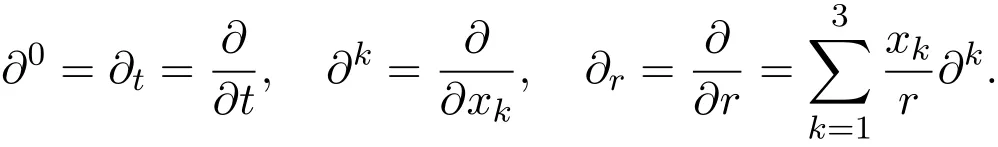
By introducing physical variable(t,x)=(t,x1,x2,x3,x4),r=|x|,define derivative

Yang-Mills potential is Aµ=Aµ(x,t)(µ =0,1,2,3),and the field functions are

where εijkis the convertible symbol and ε123=1.The covariant derivative is

For three-dimensional space vector ϕ = ϕ(x,t)(Higgs field),set ψµ=Dµϕ,then Lagrange density[3]is

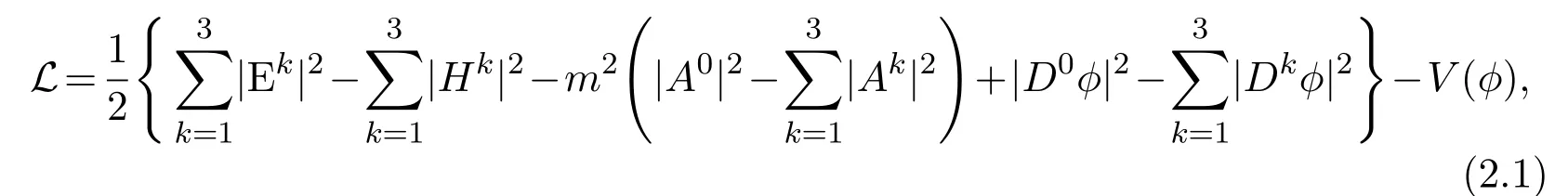
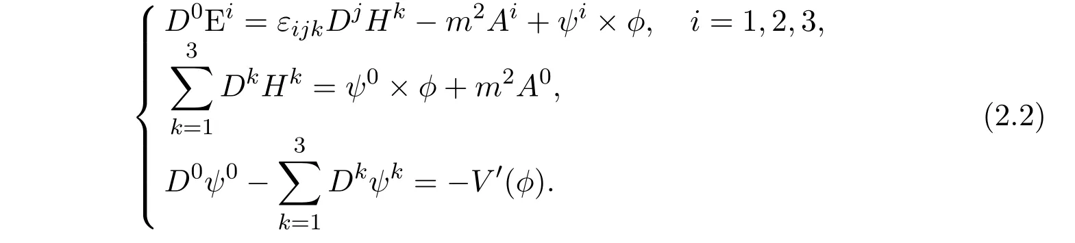
where V(ϕ)=V0(|ϕ|2),V0is a real function of real variable.Letwhereis the derivative of V,the motion equations of L has the following form:

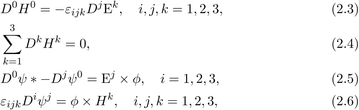
By the definitions of Ei,Hiand Jacobi identity,we can find the following equations

There is the following result.

Theorem 2.1Assume that

(i)V(ϕ)=c1|ϕ|2+c2|ϕ|4,wherec1andc2are nonnegative constants,

(ii)α0,β0∈∩,α1,β1∈,m=0,c2=0,or

(iii)α0,β0∈∩,α1,β1∈,m>0,c2>0,

thus under conditions(i)(ii)or(i)(iii),Yang-Mills-Higgs equations(2.2)-(2.6)have a unique solution satisfying

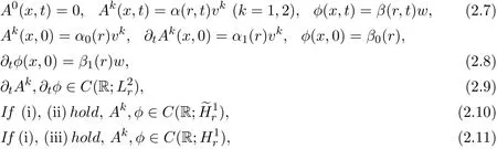
where,are radial functions ofr=|x|,having compact support,with the complete space being equaled with the norms∥∇ϕ∥2and∥ϕ∥2+∥∇ϕ∥2respectively,anddenotes the radial symmetric function inLpintegrable space.

3 Maxwell-Higgs Equation

The Maxwell-Higgs equations(also known as Ginzburg-Landau equations)takes the following form

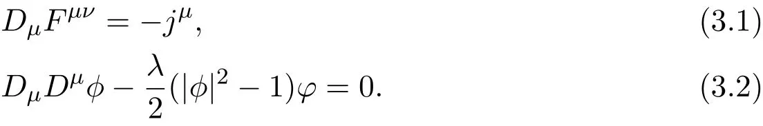
Denote the time variable t by x0and the spatial variables by xj(j=1,2,3),∂µ=∂xµ.xµare the coordinates of Minkowski space(R1+3,gµν); µ,ν =0,(gµν)=diag(−1,1,1,1),is the covariant derivative for any space or time variables,Aµis the electromagnetic potential,φ is the complex function and an order parameter of Higgs field,λ is Ginzburg-Landau constant,for simplicity,letting λ=1.

The electromagnetic field Fµνgives rise to the induced electric and magnetic fields as follows

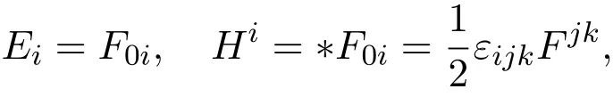
where ∗F is the Hodge dual of F,

For given function φ(x,t),we define its spatial gradient∇φ =(∂iφ)i=1,2,3,where∂φ =(∂0φ,∇φ)is the full spatiotemporal gradient.Denote D’Alembert operator by?,

It is easy to see that equations(3.1)and(3.2)have total energy conservation

where

Ginzburg-Landau equations are gauge-invariant with respect to the appropriate smooth function χ,defining

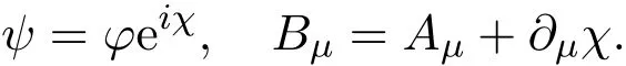
It is easy to known that if(φ,A)is the solution of equations(3.1)and(3.2),then(ψ,B)is also the solution of them.In order to make definite solutions of well-posed problem,we must add gauge conditions

(i)Coulomb gauge

(ii)Temporal gauge

In fact,if the finite energy solution exists under the coulomb gauge condition,then we can obtain the same result under the appropriate gauge transformation.Therefore,we only need to consider the coulomb gauge condition(3.3).

It’s different from the method obtained by Eardley Monerief,from which we can obtain the existence of global smooth solution to Yang-Mills-Higgs equations under the temporal gauge condition.By the method obtained by Klainerman et al.,the existence of finite energy global solution of equations(3.1),(3.2),(3.3)or(3.4)is obtained.

Under the coulomb gauge condition,the solution of equations(3.1)-(3.3)can be written as the following form

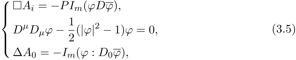
where P denotes the projection operator on a divergence field,namely,for any field B,

By∇∂0A0=0,(3.1)can be written as(3.5)1.Consider the initial condition

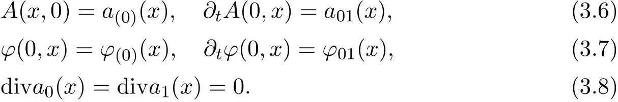
It follows from(3.5)2that

By(3.9),it yields

We know from equation(3.10)that if the initial values a0and a1are the form of divergence free,then(3.3)is automatically satisfied for all time t.

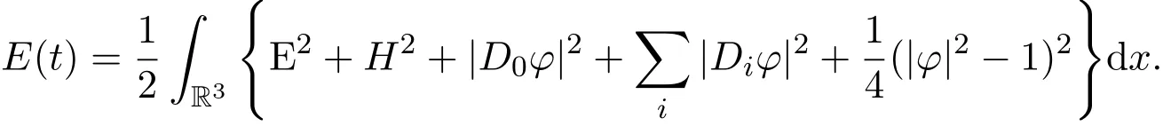
Introduce energy module

then there exists the following result.

Theorem 3.1Consider the general initial valuea(0),a(1),φ(0),φ(1),for equations(3.6)-(3.8),and let

then there exists a unique generalized solution

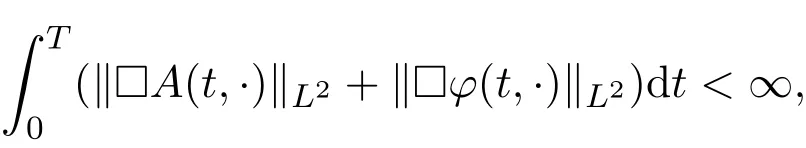
wheredenotes the homogeneous Sobolev space and satisfies the energy inequalityE(A0,A,φ)≤ F0.Furthermore,we obtain

(i)

(ii)

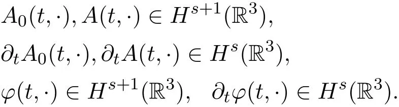
(iii)if the initial value is smooth,∇a(0)∈Hs(R3),a(1)∈Hs(R3),φ(0)∈Hs+1(R3),φ(1)∈ Hs(R3),s>0,then for anyt>0,there is

Next consider the instability of Maxwell-Higgs equations with respect to symmetric vorticity.

Consider Maxwell-Higgs equations[4]

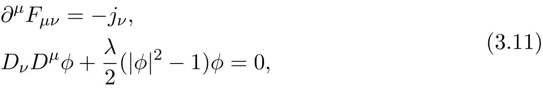
where Dµ= ∂µ−iAµ,Fµν= ∂µAν−∂νAµ,µ =0,1,2,Aµ(x)is the electromagnetic field potential,ϕ(x)is Higgs field,F0j,j=1,2 are the electric fields,−F12is the magnetic field,

The conservation of energy is

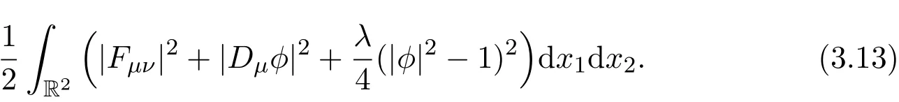
For the stationary Ginzburg-Landau equations

there is a vortex number as follows:

which has a topological significance as the winding number of the Higgs field ϕ.The numerical results indicate that for λ≤1 and all charges n,the vortices are stable.On the other hand,for λ >1 and|n|≥ 2,the vortices are unstable.We can give its analytical proof.

Under the temporal gauge condition A0=0,the Maxwell-Higgs system takes a form as follows:

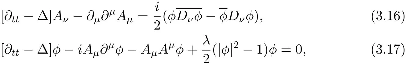
where ν,µ =0,1,2.Aµ=,µ =0,AµAµ= −,µ ≠0.We can rewrite(3.16),(3.17)as the following form:

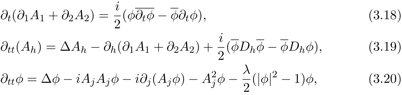
where h=1,2,j=1,2.

First we linearize the Maxwell-Higgs system around a given radial vortex(a,η)in the temporal gauge A0=0.Plug A=a+εω and ϕ = η+εψ into the Maxwell-Higgs system(2.2),(2.3),and(2.4),and take the derivative with respect to ε.Evaluating at ε=0,we obtain the linearized Maxwell-Higgs system:

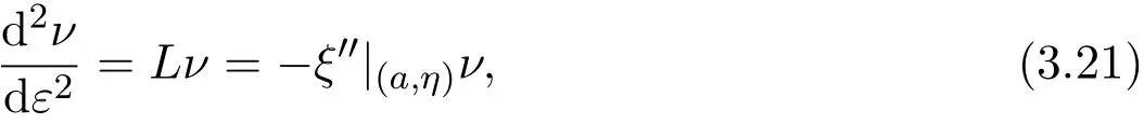
where ν =(ω1,ω2,ψ1,ψ2)T, ψ1=Reψ =Imψ.

The linear operator L has the form

where

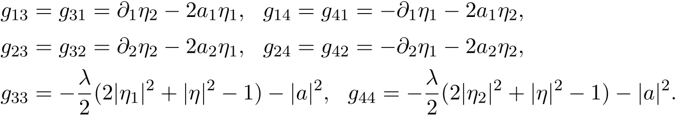
It can be proved that for the vortex(a,η)that the system is not only linear stability but also nonlinear instability in the norm ∥ν∥X= ∥ν∥H1(R2)+ ∥ν∥L∞(R2).

Theorem 3.2Let(a,η)be vortices such that

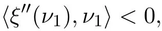
for someν1∈ H1(R2),then there exists anε0>0,c>0,for any smallδ>0there exists a family of solutionνδ(t)of the Maxwell-Higgs equations such that the vortex number ofωδ(0)is zero and

but

Thus(a,η)is unstable with the normX.

4 Einstein’s Vacuum Equation

Einstein got the following famous Einstein equation in studying the gravitational field

where Rµνis Ricci tensor,the scalar curvature R is

Tµνis the energy-momentum tensor.If k=8πG,G is the Newton’s gravitational constant,then there is Einstein gravity field equation

If k=8πG+4Λ,T=gµνTµν,there is

If there is no matter,the Einstein’s vacuum equation can be obtained,

where Λ ≥ 0 is the cosmical constant,gµνis the Riemann matrix.

Consider the following form of Einstein’s vacuum equation

where N denotes the term with the square of the first derivative∂g.Consider the initial value problem along the super-plane Σ:t=x0=v,

where∇represents the gradient with respect to the space coordinates xi,i=1,2,3.Hsis Sobolev space.Let gαβ(0)be continuous Lorentz matrix and

Theorem 4.1Assume that equation(4.5)satisfies the initial value conditions(4.6),(4.7),fors>,then there exist temporal interval[0,T]and unique solution(lorentz matrix)g ∈ C0([0,T]×R3),∂gµν∈ C0([0,T],Hs−1),Tonly depends on the norm∥∂gµν(0)∥Hs−1.

Theorem 4.2Consider the classic solution of equation(4.5),then there exists a temporal intervalTonly depending on∥∂gµν(0)∥Hs−1for any givens>2.

To show Theorem 4.2,rewrite(4.5)as

where ϕ =(gµν),N=(Nµν),gαβ=gαβ(ϕ).

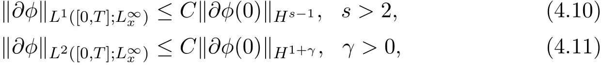
In order to prove Theorem 4.2,the following estimates need to be established:Energy estimate.For the solutions of equation(4.5),there is

where the constant C only depends on ∥ϕ∥L∞([0,T];L∞x)and ∥∂ϕ∥L1([0,T];L∞x).

By Strichatz estimate,

and bootstrap hypothesis

we can make the better estimates

5 Yang-Baxter Equation

Yang-Baxter equation is obtained by Yang when studying the S scattering matrix of multibody problem in 1967.In 1982,Baxter introduced it to the exactly solvable model in statistical mechanics,which plays an important role in the quantum backscattering method.

Yang-Baxter equation is the matrix equation of three space ν1× ν2× ν3

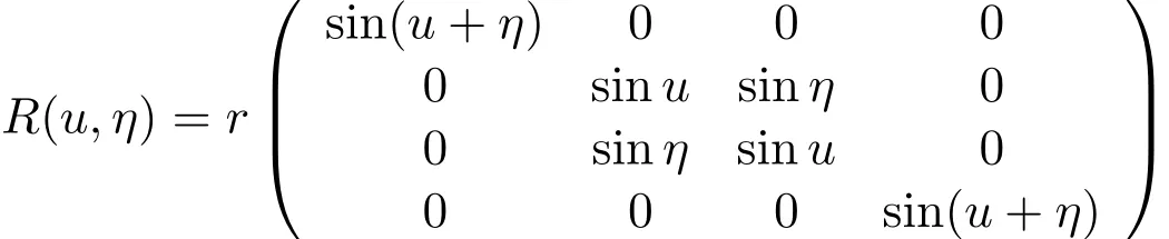
where k matrix acts only on two direct product spaces,and the action on the third space is equivalent to the identity transformation.Yang-Baxter equation contains two parameters,one is the quantum parameter η,the other is the spectral parameter u.Yang obtained Yang solution:

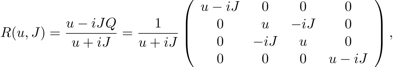
where J is the coupling constant,Q is the exchange operator of two spaces

In two-dimensional ice pole model,Quantum parameters and spectral parameters are all related to pole energy:

We obtain

or

A,B:X→X are the bilinear operators,X is a linear space.

6 Chern-Simons-Higgs Equation

Consider a nonlinear Schrödinger equation

Let ρ =|ψ(t,x)|2,then we have

Thus,if we use the notation J=(Jµ)=(ρ,Jk),where

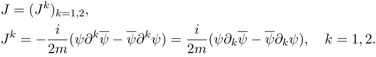
So we have

It is clear that equation(6.1)is the Euler-Lagrange equation of the action density[5]

We introduce a real-valued gauge filed A=(Aµ)(Aµ∈ R,µ=0,1,2)and covariant derivatives Dµ= ∂µ− iAµ,µ =0,1,2.Hence we arrive at the gauged Schrödinger equation

We introduce Maxwell equation

where Fµν= ∂µAν− ∂νAµ,µ,ν=0,1,2.The strength tensor gives rise to the induced electric and magnetic fields,E=(E1,E2,0)and B=(0,0,B),by the standard prescription

Therefore,(6.5)becomes

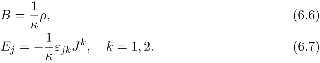
Equation(6.5)or system(6.6),(6.7)is the simplest Chern-Simons-Higgs equation.

Equations(6.4),(6.5)are gauged Schrödinger-Chern-Simons equations.It is clear that this system is the Euler-Lagrange equations of the action density

In the following we shall look for the explicit static solutions which are independent of x0=t of the nonrelativistic Chern-Simons theory(6.8),hence equations(6.4)-(6.6)become

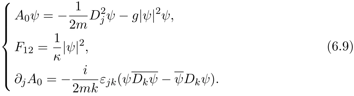
By some calculations,(6.9)can be reduced into

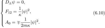
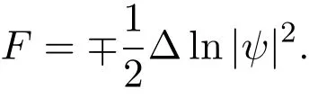
It can be shown as before that(6.10)1implies that the zeros of ψ are discrete and finite.Let the zeros be p1,p2,···,pN∈ R2.By the subtitution u=ln|ψ|2,we transform(6.10)1,(6.10)2into the equivalent Liouville equation

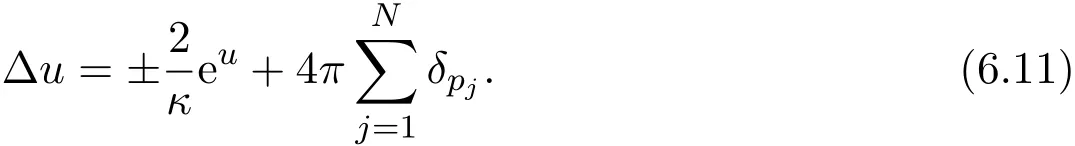
If let κ = ∓|κ|,(6.11)becomes

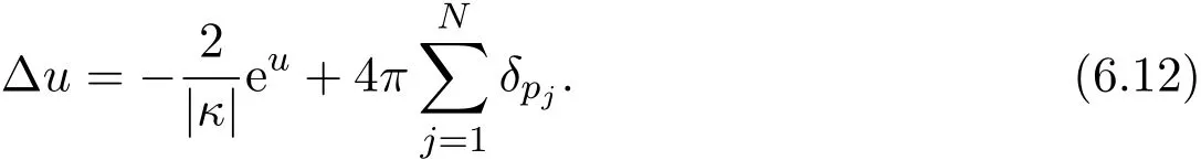
Using the complex variable z=x1+ix2and Liouville method,we can rewrite u as

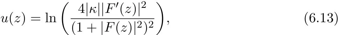
where F(z)is any holomorphic function of z so that p1,p2,···,pNare the zeros of F′(z).In particular,we may choose F(z)to be a polynomial in z of degree N+1.The solution pair(ϕ,A)of the self-dual equations are given by the scheme

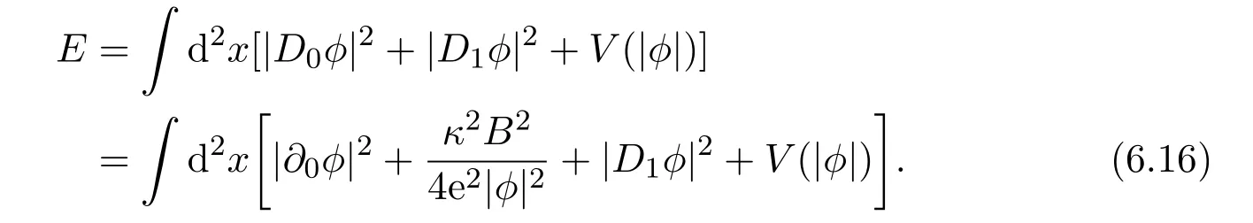
Consider Abelian Chern-Simons-Higgs system[6]

The theory possesses two vacua: ϕ =0 and|ϕ|=v,one is symmetric and the other is asymmetric.

The energy of the system is

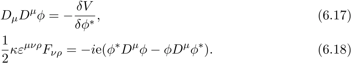
The equations of motion are

Performing the Bogomol’nyi factorization,one obtains

where D±ϕ =(D1±iD2)ϕ,then

where ΦB= ∫d2xB=2πn/e.

Consider the self-dual Maxwell-Chern-Simons Lagrange is

with the BPS potential

The Bogomol’nyi completion of the energy is

and the seld-duality equations are

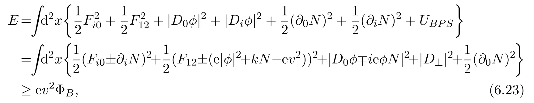
Consider the domain wall energy of system(6.21)

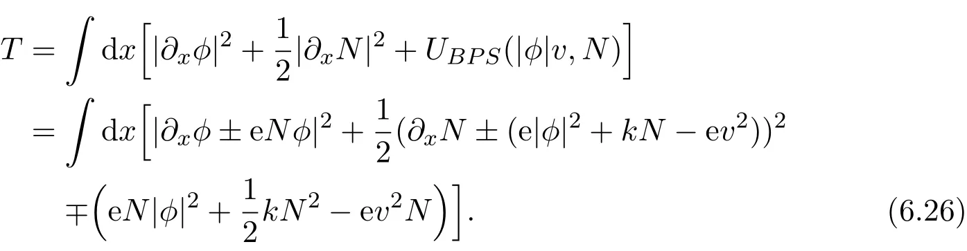
When Ax=0,the energy reads

where the Gauss law has been used to write the completion and the second set of±s is independent of the first set and is marked with′.