Numerical simulation of the climate effect of high-altitude lakes on the Tibetan Plateau

YinHuan Ao , ShiHua Lyu , ZhaoGuo Li *, LiJuan Wen , Lin Zhao

1. Key Laboratory of Land Surface Process and Climate Change in Cold and Arid Regions, Northwest Institute of Eco-Environment and Resources, Chinese Academy of Sciences, Lanzhou, Gansu 730000, China

2. Plateau Atmosphere and Environment Key Laboratory of Sichuan Province, School of Atmospheric Sciences, Chengdu University of Information Technology, Chengdu, Sichuan 610225, China

3. Collaborative Innovation Center on Forecast and Evaluation of Meteorological Disasters, Nanjing University of Information Science & Technology, Nanjing, Jiangsu 210044, China

ABSTRACT Lakes regulate the water and heat exchange between the ground and the atmosphere on different temporal and spatial scales. However, studies of the lake effect in the high-altitude Tibetan Plateau (TP) rarely have been performed until recently, and little attention has been paid to modelling of frozen lakes. In this study, the Weather Research and Forecasting Model (WRF v. 3.6.1) is employed to conduct three numerical experiments in the Ngoring Lake Basin (the original experiment, an experiment with a tuned model, and a no-lake experiment) to investigate the influences of parameter optimization on the lake simulation and of the high-altitude lake on the regional climate. After the lake depth, the roughness lengths, and initial surface temperature are corrected in the model, the simulation of the air temperature is distinctly improved. In the experiment using a tuned model, the simulated sensible-heat flux (H) is clearly improved, especially during periods of ice melting (from late spring to early summer) and freezing (late fall). The improvement of latent-heat flux (LE) is mainly manifested by the sharp increase in the correlation coefficient between simulation and observation, whereas the improvement in the average value is small. The optimization of initial surface temperature shows the most prominent effect in the first year and distinctly weakens after a freezing period. After the lakes become grassland in the model, the daytime temperature clearly increases during the freezing and melting periods; but the nocturnal cooling appears in other stages, especially from September to October. The annual mean H increases by 6.4 times in the regions of the Ngoring Lake and the Gyaring Lake, and the LE declines by 56.2%. The sum of H and LE increases from 71.2 W/m2 (with lake) to 84.6 W/m2(no lake). For the entire simulation region, the sum of H and LE also increases slightly. After the lakes are removed, the air temperature increases significantly from June to September over the area corresponding to the two lakes, and an abnormal convergence field appears; at the same time, the precipitation clearly increases over the two lakes and surrounding areas.

Keywords: Lake-surface temperature; roughness length; turbulent flux; Ngoring Lake; Tibetan Plateau

1 Introduction

Lakes regulate the water and heat exchange between the ground and the atmosphere on different temporal and spatial scales and, therefore, affect regional climate (Rouseet al., 2005; Longet al., 2007;Balsamoet al., 2012; Le Moigneet al., 2016). The surface processes and climate effects of lakes are complicated by the diversity of areas, depths, and compositions of lake water and the climate conditions (Downing, 2010; Readet al., 2012; Woolwayet al., 2016, 2017). Readet al. (2012) demonstrated that lake size influences the wind shear and convective mixing in lakes. An investigation in the Northeastern United States found that smaller lakes warmed more rapidly than larger lakes in terms of surface temperature (Torbicket al., 2016). Additionally, small lakes are often well sheltered from the wind and consequently experience lower wind speeds than large lakes with greater fetch (Hondzo and Stefan, 1993),which, also called the fetch length, is the length of water over which a given wind has blown. The nonfrozen lake usually decreases the amplitude of daily temperature variation in the lake area (Samuelssonet al., 2010), and lakes at mid or high latitudes are usually colder than nearby land in spring and summer.Lakes at middle or high latitude have an inhibitory effect in the warm season on the heat flux and precipitation over the lake surface (Lofgren, 1997; Dutraet al.,2010; Eerolaet al., 2010). Compared with the land,low-latitude lakes generally have relatively higher temperatures, which increases the regional latent-heat flux throughout the year (Dutraet al., 2010). During the turning and freezing processes in fall and early winter, the lakes can cause the surface air to become warmer and more humid (Jeffrieset al., 1999), which is conducive to the formation of lake-effect precipitation in the downwind area (Bateset al., 1993;Kristovich and Braham, 1998; Lofgren, 2004) until the lakes are frozen and covered by thick snow (Dutraet al., 2010). Conversely, during the melting period,the lakes cause the surface air to become colder(Samuelssonet al., 2010). As the Great Lakes in North America are the largest inland-lakes group in the world, lake-effect precipitation there has been considerably investigated (Norton and Bolsenga,1993; Ellis and Leathers, 1996). Based on numerical simulations, Lavoie (1972) discovered that the temperature difference between the lake surface and 850 hPa is an important factor that triggers lake-effect precipitation. The air-lake interaction can cause heavy precipitation on the downwind side, particularly during late autumn–early winter when cold air masses passing over the Great Lakes are warmed and moistened by the underlying water (Bateset al., 1993;Wrightet al., 2013). Wilson (1977) noted that the precipitation in a lake's downwind direction significantly increases when the temperature at 850 hPa is 7 °C below the lake-surface temperature. The ice cover of lakes also has an important effect on the precipitation by changing the lake evaporation and the stability of the atmosphere in the lower part of the boundary layer. Zhaoet al. (2012) employed the Moderate Resolution Imaging Spectroradiometer (MODIS) product to improve simulation of lake-effect precipitation by improving the initial lake-surface temperature in the model.

However, previous studies were concentrated in North America, northern Europe, and other low-altitude areas. Studies of the lake effect on the high-altitude Tibetan Plateau (TP) were rarely performed until recent years. The total area of TP lakes is 4.7×104km2(Zhanget al., 2013; Wanet al., 2016), which accounts for approximately half of the lake area in China. Due to an increase in the meltwater of glaciers and precipitation, the lake areas have continuously increased on the TP in recent years (Songet al., 2014;Yanget al., 2018). The Tibetan Plateau, with an average elevation of 4,500 m above sea level, has an important effect on the global water cycle and Asian monsoons, and is an area sensitive to climate change(Yaoet al., 2011; Yanget al., 2014). Solar radiation is extremely strong on the TP, whereas the air density and pressure are only 50%–60% of those at sea level,which can create a higher atmospheric convection efficiency under the same surface-heating conditions(Zhang, 2007). In recent years, observations indicate a persistent unstable atmosphere on the surface of the Nam Co Lake and the Ngoring Lake, where the water-surface temperature usually exceeds the air temperature after the lake ice melts (Biermannet al.,2014; Liet al., 2015, 2017; Wanget al., 2017). This phenomenon distinctly differs from that of other lakes at mid or high latitude. A recent study shows the frequency of an unstable atmospheric-boundary layer increases with decreasing latitude and lake-surface area(Woolwayet al., 2017). Wenet al. (2015) employed a coupled atmosphere–lake model and discovered that the lakes can decrease the annual temperature range and increase annual precipitation on the lake surface and surrounding area by 49%. However, it is difficult to describe accurately the influence of the heterogeneity of terrain and lake depth in a model because spatial resolution is coarse and the lake depth is uniform.In addition, the current roughness schemes in the lake model are primarily derived from oceanic observations under certain conditions (Zilitinkevichet al.,2001; Mahrtet al., 2003; Vickers and Mahrt, 2010;Grachevet al., 2011; Vachon and Prairie, 2013).There are still some shortcomings when these schemes are applied in lake modelling (Vachon and Prairie, 2013; Woolwayet al., 2015; Weiet al.,2016), which weakens the simulation capability of the model regarding the lake effect (Liet al., 2018).

The influence of lake ice and its freeze–thaw process on surface energy and the climate effect cannot be disregarded in high-altitude regions. Observation on Lake Erie indicates that the sensible-heat flux (H)nonlinearly decreases as the drifting ice increases on the lake surface, and the latent-heat flux (LE) linearly decreases as the drifting ice increases (Gerbushet al.,2008). Kristovich and Laird (1998) found that the nonuniform lake-surface temperature during the freezing process can significantly affect the heat exchange and the development of the convective-boundary layer. For the completely frozen lake, the ice cover can considerably reduce the H and LE (Niziolet al.,1995). However, little attention has been paid to the modelling of frozen lakes due to the lack of winter observations on the TP. Only a few studies analysed the freezing time of the Nam Co Lake (Yeet al.,2011), lake-ice structure (Huanget al., 2013), and ice melting (Huanget al., 2016) in a small TP thermokarst lake.

In this study, three experiments were carried out using the Weather Research and Forecasting Model(WRF v. 3.6.1) coupled with a lake model. These experiments were used to evaluate the simulation capability of the original WRF model for the TP lakes and the effect of model correction on lake modelling and,finally, also to reveal the influence of the high-altitude lake on the local climate. This study is organized as follows: section 2 introduces the study region, data,and method; section 3 describes the results in detail;and section 4 is the conclusion.

2 Study region, data, and methods

2.1 Study region

The Ngoring Lake, with an area of 610 km2, is located in the source region of the Yellow River on the eastern TP. The average depth is 17 m (with a maximum depth of 32 m), and the surface elevation is approximately 4,270 m. Gyaring Lake (526 km2) is located 15 km west of the Ngoring Lake; and the two lakes are separated by mountains. They are the highest, large freshwater lakes in China and are surrounded by low hills with alpine meadows. The multiyear average (1953–2012) air temperature and precipitation are -3.7 °C and 321.4 mm in this region.

2.2 Data

The observational data in this study include daily average air temperature, wind speed, and daily accumulated precipitation at the gradient tower station(TS) at the Ngoring Lake and at the Madoi Meteorological Station (MS), and the daily average turbulent flux on the lake-surface station (LS). The TS is located 30 m west of the lakeshore of the Ngoring Lake (34.906°N,97.568°E). The LS stands on the northwestern part of the Ngoring Lake (35.026°N, 97.652°E), 200 m from the northwest lakeshore. Water depth within 200 m around the LS ranges from 3 to 5 m. The southeast side of the LS faces the centre of the lake. The turbulent fluxes are measured at the 3.0-m height. The TS is approximately 15 km from the LS. MS is located 30 km to the east of the Ngoring Lake (34.921°N,98.211°E; 4,279 m a.s.l.). Data from TS and MS begin in May 2011 and end in September 2012, whereas the observation at the LS exists only in summer and autumn of 2011 and 2012.

2.3 Model description

The model used in this study is the WRF3.6.1 with a built-in lake model (a 1-D lake model), which can reproduce the diurnal variation of lake temperature and was released in August 2014. The built-in lake model, named LISSS (Subinet al., 2012), was obtained from the CLM4.5 (Olesonet al., 2013) with some modifications by Guet al. (2015). It is a one-dimensional mass-and-energy balance scheme with 20–25 model layers, including up to 5 snow layers on the lake ice, 10 water layers, and 10 soil layers at the lake bottom. For the ice-free lake, the energy transport can be divided into two parts (surface-layer heat exchange and subsurface-layers heating) (Xuet al.,2016). For the lake-surface layer, the surface temperature at the first time step is obtained from the air temperature, and the next time-step surface temperature and the subsurface-layers temperature are calculated by the governing equation of the lake model (Xuet al., 2016). The lake-surface roughness lengths are dynamic in LISSS and vary with the Charnock coefficient and the friction velocity (Subinet al., 2012), but they are constants in WRF (0.001 m) for ice-free lakes. The sensible-heat and latent-heat flux are calculated as by Olesonet al. (2013):

whereρis the air density,θsandθaare the potential temperature of the lake surface and air at reference height,qsis the saturated specific humidity at the lake surface,qais the specific humidity of air,rahandraqare the aerodynamic resistance to sensible-heat and latent-heat transfers,Cpis the specific heat capacity of air at constant pressure, andλis the latent heat of vapourization or sublimation.

In the triple-nested domains (Figure 1), the outermost nested domain included the TP and its surrounding region; and the third one (d03) included Ngoring Lake and the surrounding region. The parameters of the nested domains are listed in Table 1.The high-resolution simulation with the 2-km grid spacing in the innermost nested domain can describe the influence of heterogeneity in the terrain and lake depth on the simulation. The simulation experiments began on May 1, 2011 and ended on October 1, 2012(Universal Time Coordinated); and the simulation results were output every three hours for the d03 domain.In this study, the ERA-Interim reanalysis data with 1.0° spatial and 6-h temporal resolution, were employed as the initial fields and lateral boundary conditions for the outermost domain. The model was divided into 30 layers and topped at the 50-hPa level in the vertical direction. Other model parameters included the Noah land-surface model (Chen and Dudhia, 2001), the WSM6 microphysical scheme (Hong and Lim, 2006), the RRTMG long-wave and shortwave radiation schemes (Cloughet al., 2005), the MM5 similarity surface-layer scheme, and the ACM2 boundary-layer scheme (Pleim, 2007). The Kain-Fritsch cumulus scheme (Kain, 2004) is used only in the outermost (d01) and intermediate (d02) nested domains because the cumulus scheme is used mainly for coarser grid sizes (Skamarocket al., 2005). In finescale simulations, the convection may be resolved by the grid; and thus a cumulus scheme may no longer be needed (Nasrollahiet al., 2012). Li and Pu (2009)demonstrated that using a cumulus scheme at a 9-km grid size improved the simulation results, while this scheme had a small impact on the result at a 3-km grid size.

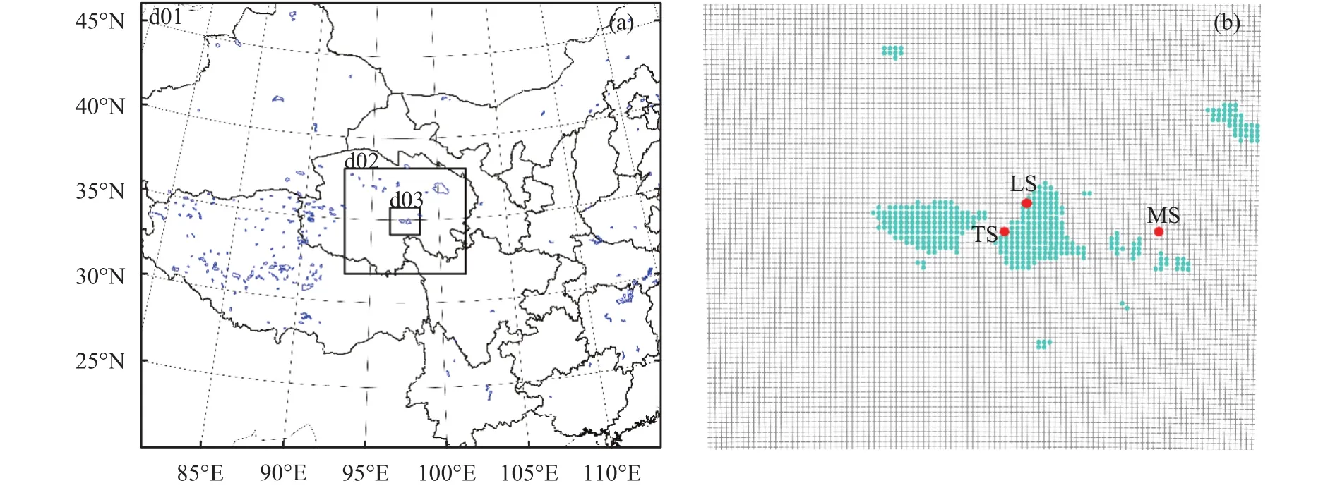
Figure 1 Domain of the WRF model simulations (a) and the horizontal discretization of the d03 domain (b): the blue lines (a)and the green grids (b) represent the lakes. Three stations (TS, LS, and MS) are marked in Figure 1b

Table 1 Parameters of grids in the nested domains

In this study, three experiments were designed:

(1) The first experiment was carried out using the original WRF v3.6.1 model without any modification(Case 1). The lake-surface roughness lengths for momentum, heat, and water vapour were equal (1 mm)during the ice-free period. The depths of the Gyaring Lake and the Ngoring Lake were 17 m and 0.5 m, respectively. The surface temperature in the initial field was derived from ERA-interim data.

(2) In the second experiment (Case 2), the observed roughness lengths for momentum (6.17×10-4m), heat (7.59×10-5m), and water vapour(6.73×10-5m) were introduced into the model (Liet al., 2016). The depths of the Gyaring Lake and the Ngoring Lake in the d02 and d03 domains were also corrected (Figure 2). The revised surface temperature in the initial field adopted the MODIS 1-km surfacetemperature/emissivity eight-day composite product(MOD11A2) from May 1, 2011 to May 8, 2011.

(3) The third experiment was the no-lake condition (Case 3). The Gyaring Lake and the Ngoring Lake were modified to be grassland; and the relevant variables, such as soil type, vegetation coverage, albedo, and surface temperature, were all revised according to the neighbouring area. The corrections of surface temperature and roughness lengths (except for the Gyaring Lake and the Ngoring Lake) in Case 3 were the same as in Case 2.

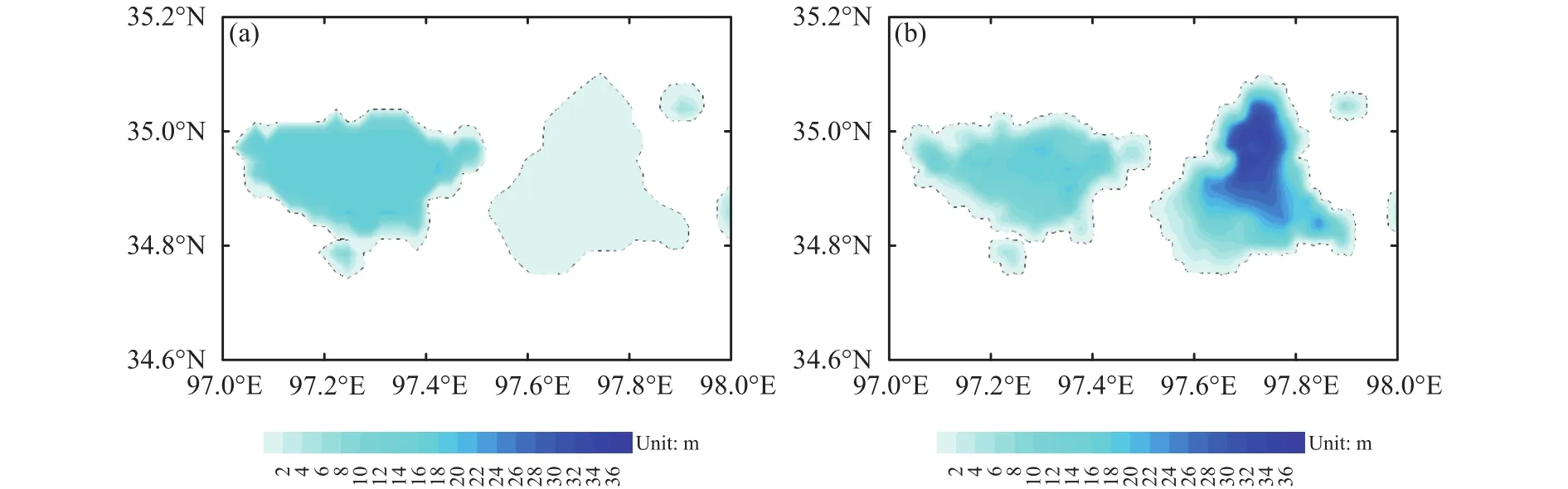
Figure 2 Original (a) and improved (b) lake depths of the Gyaring Lake (left) and the Ngoring Lake (right) in the d03 domain in the WRF model

3 Results and discussions

3.1 Evaluation of simulated results

3.1.1 Temperature, wind speed, and precipitation

The simulated results from the d03 domain were analysed. The average values of two grids in the Ngoring Lake closest to TS, with a lake-surface grid and a land grid, were employed to compare with the observation of TS. The underlying surface at Madoi is relatively uniform; we adopted the result of a single grid.

Observed and simulated half-monthly average air temperature and wind speed are presented in Figure 3.Both Case 1 and Case 2 can adequately simulate the annual variation of air temperature. However, from November to the next April, the simulated temperature was relatively low at the Ngoring Lake and the Madoi Station; and the wind speed at the Madoi Station was clearly higher. The mean value, correlation coefficient, and root mean square error (RMSE) of the simulation and observation are listed in Table 2. The precipitation observation occurred only in summer and autumn at the Ngoring Lake, where the effective period for the precipitation observation was 158 days.During this period, the accumulative precipitations for the observation, Case 1, and Case 2 were 390.2,621.7, and 604.0 mm for the Ngoring Lake, respectively. The simulation values were clearly higher, and Case 2 was closer to the observation. At Madoi, the effective period of precipitation observation was 460 days. The accumulative precipitations for the observation, Case 1, and Case 2 were 735.9, 799.9, and 901.4 mm,respectively. Case 1 was closer to the observation(Figure 4).

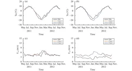
Figure 3 Observed and simulated half-monthly average air temperature and wind speed for the Ngoring Lake(a, c) and the Madoi Station (b, d) in Case 1 and Case 2

Table 2 Correlation coefficient, root mean square error (RMSE), and mean of air temperature and wind speed for the simulation and observation

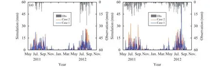
Figure 4 Observed and simulated daily precipitation in Case 1 and Case 2 for the Ngoring Lake (a) and the Madoi Station (b)

Figure 5 shows the spatial distribution of the precipitation and wind field at 550 hPa in Case 2, as well as the difference between Case 1 and Case 2 (Case 1 minus Case 2). Note that the study period in 2011 covered June 1 to October 31 (five months), and the period in 2012 covered June 1 to September 30 (four months). We eliminated the simulated result that is adjacent to the domain border when plotting the figure, to avoid model artefacts near the lateral boundaries (Maussionet al., 2011). The precipitation exhibited a distribution pattern of more in the south and less in the north. South of the Ngoring Lake and the Gyaring Lake basins is a mountain area, where the elevation is higher than the lake surface by 400–500 m.The prevailing northerly wind uplifts on the windward slope of the mountain and increases the precipitation in summer and autumn. The two lakes are located in the region with less precipitation (300–500 mm),and the amount was similar to Madoi. Compared with Case 2, the amount of precipitation was less in most regions of Case 1 (Figures 5b and 5d). The difference between the two years for the region of reduced precipitation is related to the atmospheric circulation variation. For instance, an abnormal southwesterly wind appeared over the southern extent of the two lakes in 2012 (Figure 5d). Due to decreasing elevation from south to north, the abnormal downhill wind was not conducive to the formation of precipitation.

Both simulated air temperatures were lower than the observation at two stations; and in particular, they were lower by more than 1.3 °C at Madoi. The simulated temperature in Case 2 was closer to the observation, and the simulated values increased by 0.26 °C and 0.05 °C at the Ngoring Lake and Madoi, respectively. Apparently, the improvement in the initial field of the model can obviously improve the simulation of the lake basin. For the Ngoring Lake, the RMSE in Case 2 was slightly larger than that in Case 1; they are almost equal at Madoi. The simulated wind speed in Case 1 and Case 2 was only slightly higher (by 0.22–0.33 m/s) than the observation at the Ngoring Lake; but it was considerably higher at Madoi (approximately 1.9 m/s). In addition, the observed wind speed at Madoi was distinctly lower than that at the Ngoring Lake, especially in winter (Figures 3c and 3d), which may have been caused by the lower roughness length of the lake surface.

3.1.2 Sensible-heat and latent-heat flux

As previously mentioned, the simulation and observation of the conventional meteorological variables at the Ngoring Lake had a relatively satisfactory consistency. However, compared with Case 1, the improvement in air temperature and wind speed was not enough in Case 2. Due to the large spatial heterogeneity and the sparseness of observation stations, the validation of simulated precipitation had a few limitations. The sensible-heat (H) and latent-heat (LE)fluxes are also key variables in the land-surface processes modelling, which characterize the descriptive capability of the heat and water-vapour transfer at the air–lake interface.

Figure 5 Simulated precipitation amount in the summer and fall seasons and the wind field at 550 hPa in Case 2(a, c) and the difference between Case 1 and Case 2 (b, d)

Compared with Case 1, the variation trend of simulated H in Case 2 was more consistent with the observation. The observations came from LS, and the simulation results were derived from the corresponding grid. The correlation coefficients between them in Case 2 and Case 1 are 0.29 and -0.15, respectively,during the observation period. The averaged H of Case 1, Case 2, and the observation are 13.80, 23.94,and 24.81 W/m2, respectively. Apparently, the simulation of H in Case 2 was distinctly better than that in Case 1, especially in the following critical periods.From the May 1 to the June 12, 2011, the lake surface temperature (LST) in Case 1 was always below 0 °C, which means the lake was still frozen. A negative temperature gradient appears due to warm air and cold lake surface, which creates a negative H. Most of the lake ice had melted in Ngoring Lake in late April,and the positive H appeared in early May. Case 2 reproduced this phenomenon using the MODIS surface temperature. From October, the LST in Case 1 rapidly declined and was even below the freezing point at night, due to shallow water depth (0.5 m) and small thermal capacity. The temperature difference at the water–air interface rapidly decreased and even became negative, and the negative H reappeared. In Case 2, the water depth at LS was 8 m; the deeper a lake is, the larger the thermal storage; as a result, the lake did not begin to freeze until early November(Figure 6c). In the observation, the strong and positive H lasted until the freezing date in early December on the lake surface. Therefore, there is still room for further improvement in Case 2. During the frozen period, the simulated H in Case 1 and Case 2 was almost negative, which was a bit different from the observation, in which the weak positive H was also ubiquitous during the frozen period. In the simulation experiments, the H was restored to the positive value until mid-June of the next year.

Compared with the observation, the simulated LE in Case 1 and Case 2 was relatively high in summer.During the observation period (251 days), the correlation coefficients between Case 1, Case 2, and the observation are 0.24 and 0.62, respectively. The average LE for them were 112.04, 109.66, and 73.09 W/m2,respectively. The simulation for LE in Case 2 was slightly better than that in Case 1. Although the daily average LST in the summer of 2012 was similar in the two experiments, even slightly higher in Case 2, the simulated LE in Case 2 was significantly lower than that in Case 1, which is related to the daily variation amplitude of LST. The LST in Case 1 had higher maximum temperature in mid-July of 2012, compared with Case 2. The saturated water-vapour pressure exponentially increases with LST. Therefore, the saturated water-vapour pressure difference was high-er in Case 1 and created stronger LE. As shown in Figure 6c, the simulated LST was relatively satisfactory in Case 2 in late spring, early summer, and fall of 2011, primarily due to the improvement of surface temperature and lake depth.

Figure 6 Observed and simulated sensible-heat (H) and latent-heat flux (LE) on the lake surface for Case 1 and Case 2, and the daily average lake surface temperature (LST)

3.2 Influence of lakes on the regional climate

Generally, Case 2 had a better simulation result for Ngoring Lake. Therefore, Case 2 was considered as the with-lake experiment; and Case 3 (Ngoring Lake and Gyaring Lake removed) was designated as the no-lake experiment—so that we could investigate the influence of two large lakes on regional climate.

3.2.1 Air temperature and wind speed

The climate effect of lakes has a clear difference during daytime and night. In this study, the nighttime included four points of 23:00, 02:00, 05:00, and 08:00; and the daytime included four points of 11:00,14:00, 17:00, and 20:00 (Beijing time). The data in the model output corresponding to the locations of Ngoring Lake (TS) and Madoi (MS) were selected.With the exception of May 2012 (when it was higher by 0.24–1.06 °C), the half-month averaged nighttime temperature at Madoi was lower than that at the Ngoring Lake; the difference exhibited a seasonal variation (Figure 7a), and the maximum reached 2.91 °C.Normally, the temperature differences between Madoi and Ngoring Lake are largest in January–March and August–October, with that at Madoi lower by approximately 2 °C. However, the nighttime difference was small from April to June and before or after November. The endothermic process of ice melting slows the increase of air temperature in the lake area from April to June. During the daytime, the air temperature at Madoi was not always on the high side. From September to the next April, the daytime temperature at Madoi was lower than that at Ngoring Lake (0.5 °C on average); and it was higher in the other period,with the largest difference appearing from May to June (higher by 0.8 to 2 °C).

After Ngoring Lake and Gyaring Lake were removed (the no-lake condition), with the exception of late November to early December 2011 and the second half of May 2012, the nighttime air temperature decreased in this region, especially in September and October (a decrease of 1.83 to 2.09 °C), when the H on the lake surface was also the largest of the year.At Madoi, the temperature variation was small; and it was not consistent with that at Ngoring Lake after the two lakes were removed. In daytime, the air temperature distinctly increased at Ngoring Lake in Case 3, especially from November to December 2011 and from May to June 2012; and the largest magnitude of temperature increase can exceed 3 °C. Similarly, the airtemperature change was relatively small between Case 2 and Case 3 at Madoi. The nighttime wind speed ranged from 3.0 to 5.5 m/s at Ngoring Lake and from 2.0 to 4.5 m/s at Madoi. The wind speeds in the daytime were generally highest in winter (approximately 9 m/s) and lowest (less than 5 m/s) in late spring and fall. The previous analysis indicated that the simulated wind speed presented a significantly high bias at Madoi in winter and was relatively satisfactory at the Ngoring Lake. In Case 3, the nighttime wind speed had a significant variation in the lake area and consistently declined. The decreasing amplitude was relatively slight from January to May (0.5 m/s) and greatest in summer and fall seasons (1.0–2.09 m/s). In daytime, the wind speed exhibited a downward trend in the lake area during summer and fall seasons; and there was a swing trend in other times. Similar to the air temperature, the variation of wind speed at Madoi was relatively small between the two experiments(Case 2 and Case 3).

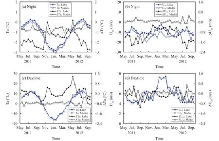
Figure 7 Simulated average temperature and wind speed (half-month average) in Case 2 and the difference between Case 2 and Case 3 (△Ta: Case 3–Case 2). The solid circle and open circle indicate Case 2 and Case 3, respectively,and the triangle symbols show the difference between two cases

3.2.2 Sensible-heat and latent-heat flux

After the lake became grassland (Case 3), a significant change of H could be observed (Figure 8a). In Case 2, the peaks of monthly average H appeared in October on the lake. However, for H in Case 3, it's almost the smallest time of the year. Moreover, the H in the two cases were closest in October. In Case 3, the maximum monthly average H was found in May(117.79 W/m2), when the H on the lake was negative in Case 2 (-7.18 W/m2), and the difference in H was most significant between them. If the period from June 2011 to May 2012 is defined as an entire year,the annual average H in the two-lakes area are 9.13 W/m2and 67.36 W/m2in Case 2 and Case 3, respectively;and the latter is 7.37 times the former. However, for the d03 domain, the difference of H in the two cases was small because the proportion of lakes in the d03 was limited. With the exception of July 2012, the H in Case 3 was consistently higher than that in Case 2;and the largest difference for monthly average H was 8.31 W/m2. The pattern of LE was opposite to that of H. After the lake became grassland, the LE decreased in each month. The difference in LE was significant in summer and fall seasons, and small in winter. From June 2011 to May 2012, the average LE in the twolakes area were 62.10 W/m2and 27.22 W/m2in Case 2 and Case 3, respectively. The latter was 43.83% of the former. With the exception of May and June 2012,the LE in Case 3 was consistently lower than that in Case 2.

As previously stated, H increased and LE decreased after the two lakes were removed. From June 2011 to May 2012, the sums of H and LE in the area of the two lakes were 71.23 W/m2and 84.58 W/m2in Case 2 and Case 3, respectively, which indicated that the total amount of heat and water exchange increased when the lakes were removed. For the d03 domain, the sum of H and LE ranged from 77.22 W/m2in Case 2 to 78.54 W/m2, with a slight increase.

3.2.3 Precipitation

Figure 9 shows the spatial distribution of accumulative precipitation from June to September in Case 2 and the difference between Case 3 and Case 2. In Case 2, the precipitation exhibited an unbalanced distribution, more in the southern area and less in the northern, with the two lakes located in the region that experienced less precipitation. After the lakes were removed, the precipitation distinctly increased over the lakes' former location and the surrounding area,with the enhancement generally exceeding 50 mm. In some areas, it even exceeded 175 mm. In 2011, the in-creased precipitation was concentrated in the area from east of Gyaring Lake to east of Ngoring Lake. In 2012, the increased precipitation appeared in the region of central-north Ngoring Lake and Gyaring Lake, and west of Gyaring Lake. The interannual difference in the region of increased precipitation was primarily related to variation in atmospheric circulation.

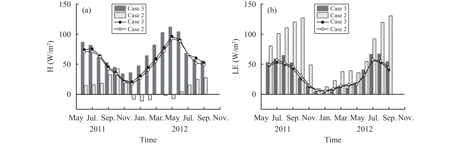
Figure 8 Monthly average sensible-heat and latent-heat fluxes in Case 2 and Case 3. The lines are the H and LE in the d03 region, and the columns are the H and LE in the area of the two lakes

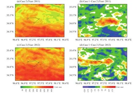
Figure 9 Simulated accumulative precipitation amount in Case 2 for 2011 (a) and 2012 (c) (from June 1 to September 30)and the difference between Case 3 and Case 2 during the same period (b and d)

From June to September, a northerly wind prevailed in the northern part of the d03 domain (Figures 10a and 10c). It gradually turned into a northeasterly wind at the two lakes. It was prone to form a convergence of wind speed in the southern mountainous region. As for the air temperature, it was relatively warm in the south and cold in the north and the two lakes. In Case 3, the warming was distinct over the two-lakes area, especially in 2012, with the average air temperature at 550 hPa increasing by 0.15 to 0.30 °C.An abnormal convergence wind field formed over eastern the Gyaring Lake to southern the Ngoring Lake in 2011 (Figure 10b), and moved northward to the central north of the two lakes in 2012 (Figure 10d), which was consistent with the region of increased precipitation (Figure 9). After the lakes were removed, the warming of ground and air, as well as the appearance of the abnormal convergence wind field, was conducive to the enhancement of precipitation.

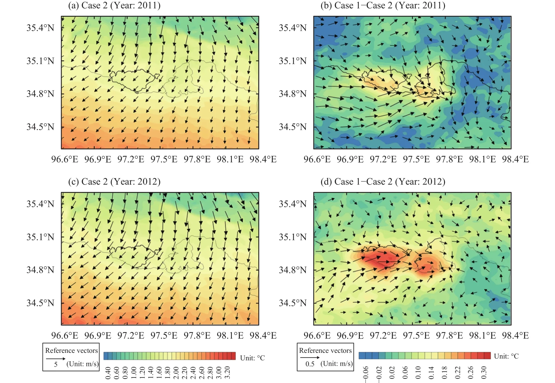
Figure 10 Simulated air temperature and wind field at 550 hPa for 2011 (a) and 2012 (c) in Case 2 (from June 1 to September 30),and the difference between Case 3 and Case 2 during the same period (b, d)

4 Conclusions

In this study, a tuned WRF3.6.1 Model using three experiments (the original experiment, the experiment with a tuned model, and the no-lake experiment) was employed to study the effect of model correction on the lake simulation and the effect of high-altitude lakes on regional climate. The main conclusions are as follows:

(1) After the lake depth, the roughness length, and initial surface temperature in the model were corrected, the simulation of air temperature over the lake was distinctly improved. The simulation of the sensible-heat flux at the lake surface was also improved,especially in the periods of ice melting and freezing.The improvement of latent-heat flux was primarily manifested by a sharp increase in the correlation coefficient between the simulation and observation,whereas the improvement in the average value was relatively small. Correction of the initial surface temperature was mainly reflected in the first year, and the effect distinctly weakened in the ice-free period of the following year.

(2) When the lakes were removed and their area became grassland in the model, the daytime warming mainly appeared in the periods of freezing and melting; and night-time cooling was found in the other period, especially from September to October. In the area of the two lakes, the sensible-heat flux increased by a factor of 6.4; and the latent-heat flux declined by 56.2%. The sums of H and LE increased from 71.2 W/m2(with lake) to 84.6 W/m2(no lake). After the lakes were removed, warming occurred over their former locations from June to September, with an abnormal convergence field appearing. The precipitation increased over the two lakes and surrounding areas,whereas the precipitation generally decreased in other regions. The interannual variations of the convergence field were consistent with the region of increased precipitation.

Acknowledgments:

This research was supported by the National Natural Science Foundation of China (Nos. 91637107,41605011, 41675020, 91537214 and 41775016),Sino-German Research Project (No. GZ1259), the Science and Technology Service Network Initiative of CAREERI, Chinese Academy of Sciences (No. 6516-71001). We acknowledge computing resources and time at the Supercomputing Center, Big Data Center of CAREERI, CAS, and GuoHui Zhao for their help with numerical simulations. We thank American Journal Experts (AJE) English-language editing for their valuable assistance with the manuscript.