Model-Based Adaptive Predictive Control with Visual Servo of a Rotary Crane System
Zhi-Ren Tsai and Yau-Zen Chang
Abstract—This paper investigated the implementation of an adaptive predictive controller using nonlinear dynamic echo state neural (ESN) model for a rotary crane system by the visual servo method.The control sequences within the control horizon were described using cubic spline interpolation to enlarge the predictive horizon. Verification of the proposed scheme in the face of exogenous disturbances and modeling error with inaccurate string length was demonstrated by both simulations and experiments.
1. Introduction
Many papers in the field of stereo vision[1]-[6]have been published in the past decade. The progress has been made in improving accuracy as well as achieving real-time performance by using multiple cameras. However, using cameras to compute 3D position coordinate of targets is still challenging due to the unpredictable lighting conditions, unavoidable noise,and interferences of the surrounding objects.
In this paper, the proposed rotary crane system is equipped with a camera for payload monitoring. This arrangement is important and novel in building construction, factories, and harbors as it avoids the installation of durable encoders at the hanging base of string. To achieve the reliable position estimation, a white light emitting diode (LED) is attached on the payload and a camera is installed on the rotary frame to derive swing angles for control feedback. The model predictive control (MPC)[7],[8]is applied on this system. Importantly, the motors in the system are controlled in velocity mode, which much simplifies the consideration of nonlinear effects caused by friction and load. Furthermore, to compensate for the timedelay effects in visual servo, a robust adaptive predictive controller is proposed by using echo state neural (ESN)network[9],[10].
2. 3D Modeling by a Camera
The coordinate systems are shown in Fig. 1. The coordinate transformation of the coordinates attached on the rotary crane and the camera as in Fig. 1, is defined as follows:
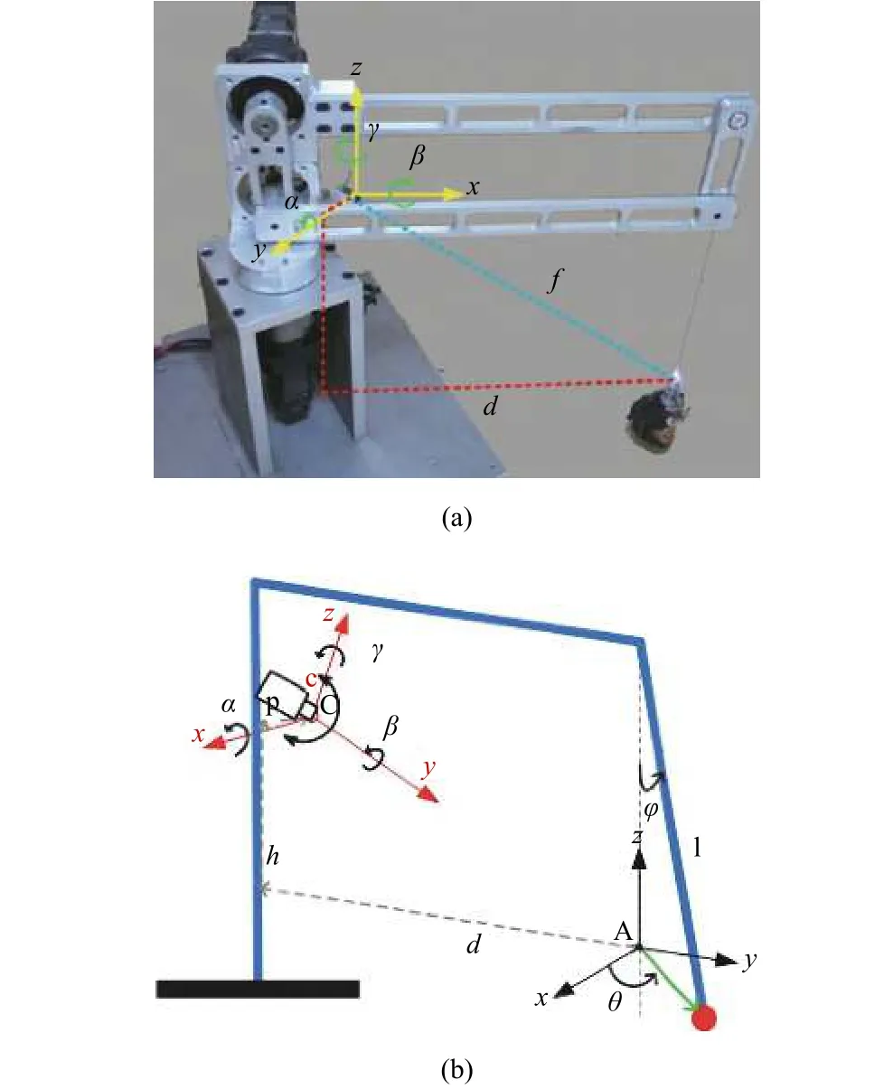
Fig. 1. Coordinates of the proposed rotary crane: (a) picture of the crane system showing the coordinate systems and (b) schematic diagram of the coordinate systems.

For the camera coordinate system, as shown in Fig. 2, there are an image planeπand a camera frame center O. The distance between O andπis the focal lengthf, and the projective pointpis the intersection of the line connecting point P and O with the image planeπ. By the properties of similar triangles, the 2D image coordinate is calculated as follows:

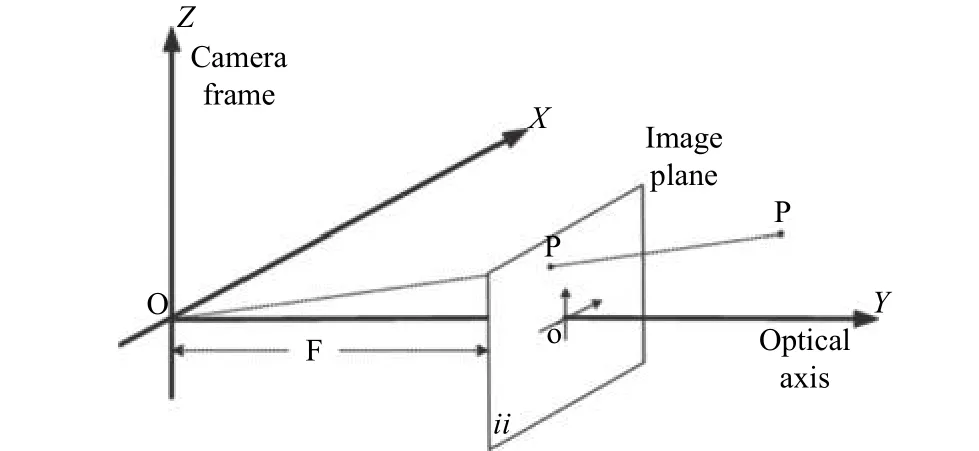
Fig. 2. Coordinate of the camera.
In order to find the solutions ofof this 3D position coordinate model, the downhill simplex method is used with the experimental measurements served as training data, as listed in Table 1. The results are shown in Table 2. Next, considering that

Table 1: Relationships between and using experimental measurements
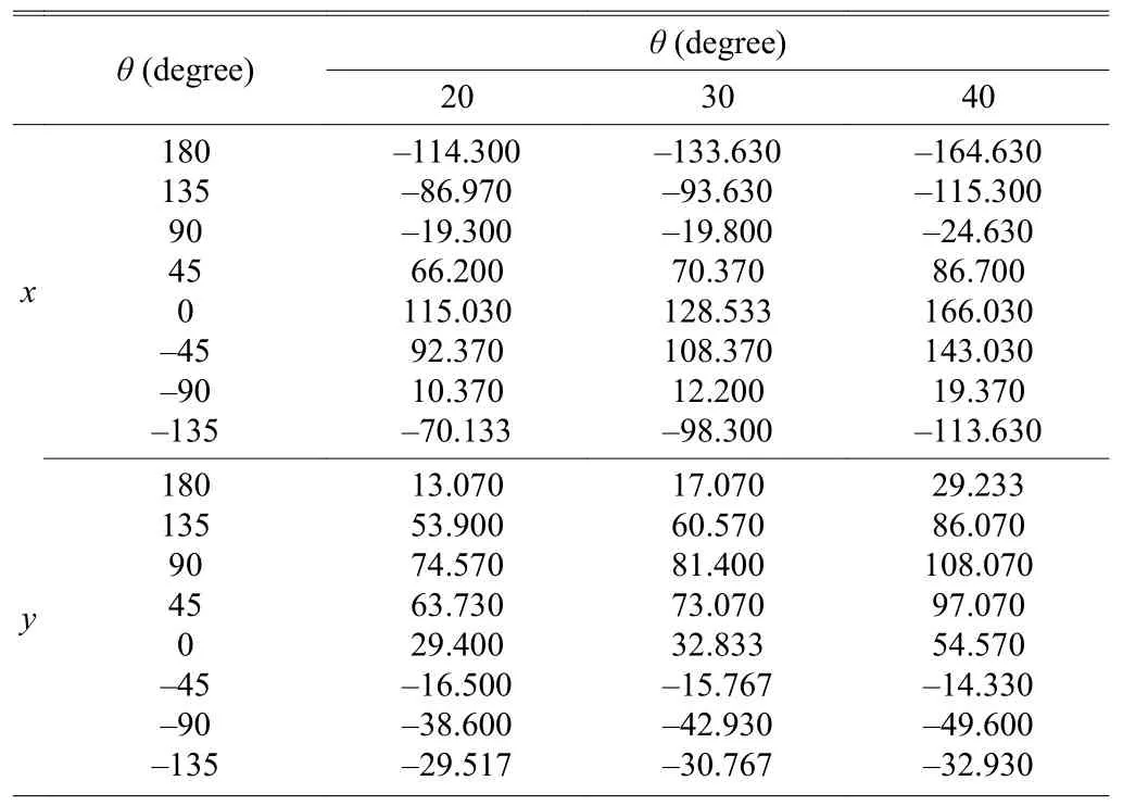
Table 1: Relationships between and using experimental measurements

Table 2: Optimal device parameters of the rotary crane and the camera
Moreover, we notice that the position of the swinging load can be uniquely defined byand, as shown in Fig. 3. Hence,we use the Kriging algorithm to find the 3D Kriging surface model for interpolating 3D coordinates, usingas input,for the purpose of minimizing the visual delay, as shown in Fig. 4.
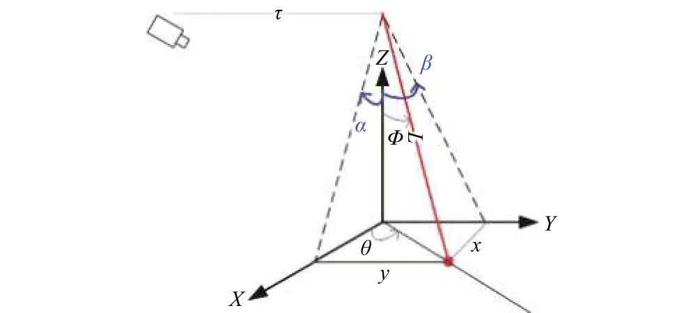
Fig. 3. Definition of swinging angles.
3. Predictive Control
In this section, a general scheme of Fig. 5 is proposed in the predictive control to extend the control horizon for more than one step in order to compensate for the delayed sensor feedback using a camera[7],[8],[11].
The physical model of the rotary crane system is described as follows:
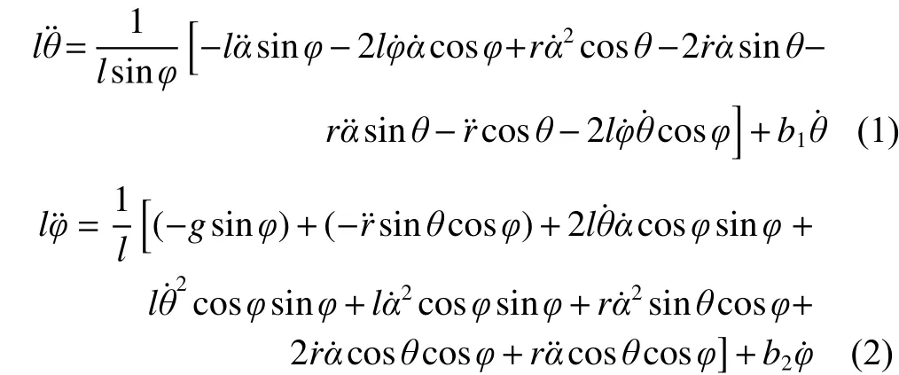
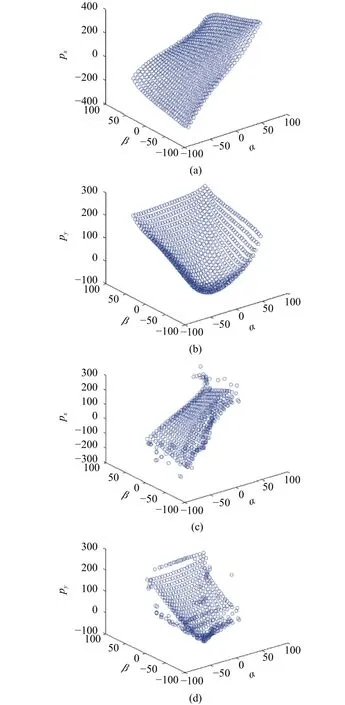
Fig. 4. Model of position and swinging angles: (a) and (b) are the model between the position () and the swinging angles α and β, respectively; (c) and (d) are the 3D Kriging surface fitting model for the position () and the swinging angles α and β,respectively.
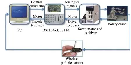
Fig. 5. Control structure of this study.

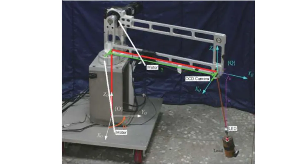
Fig. 6. Picture of the experimental prototype setup.
During the time interval betweenand, the ESN-model-based controllersimulates a physical model described by:

using estimated initial state vector, where,is sampling period and;is the prediction horizon, andis the desired output of model output.Relations between these variables and parameters are shown in Fig. 7.
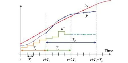
Fig. 7. Relations between the reference trajectory, candidate control inputs, and estimated system output during the predictive control.


4. Real-Time Implementation
In this section, a tapped-delay[12]ESN network[13]-[15]is designed as an adaptive model for cubic spline interpolation[16],[17]to enlarge the predictive horizon[18],[19], where the physical model-based controller[20]in (4) is replaced by a discrete-time ESN mode composed of 10 neurons each equipped with 9 tapped-delay.
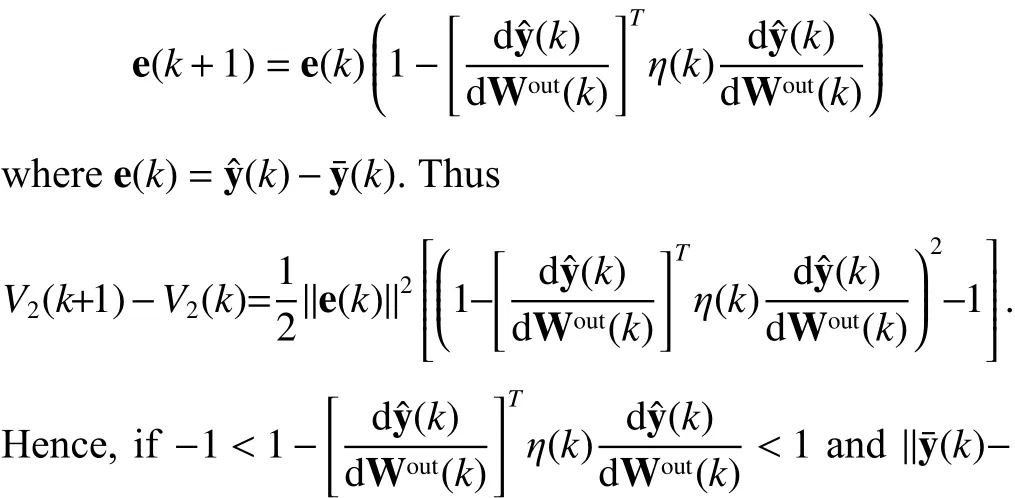
Furthermore, an adaptation theorem is used for modeling to enhance the accuracy of ESN-based model. First, the input sequence is assumed to be amatrix, ESN hasNneurons and the output is anmatrix, moreover, the state of each neuron is, where the length ofis anmatrix,isand theis. The final outputs of model is
To complete the neural plant modeling design, a convergence theory for this model is provided in the following theorem:

Proof of Theorem 1.First, the Lyapunov candidate[21]is designed as follows,

.
This model is then trained such thatis minimized.The following derivation involves a convergence condition for selecting appropriate learning rates. Firstly we notice that, we have that. This is equivalent to, thereby the proof is completed.
Input to the ESN model are past positions, velocities, and accelerations of motor and payload. Outputs of the ESN model are now positions of payload. Each trial control sequence is encoded into 3 parameters which define a cubic spline.
In order to find the best solution on-line, the downhill simplex method is used. Considering that the method suffers from the possibility of being trapped in local minima, we restart each interval with four polytopes of 4 vertices randomly and make it calculate for 20 iterations, and then start a polytope with the 4 best results of these polytopes as vertices and run for 20 more iterations.
5. Experimental Verification
Experimental prototype of Fig. 6 was used for several verification experiments. In the experimental settings, the cable length varies between 0.175 m and 0.400 m, and the payload is assumed to be 2.851 kg hanging from a cable of 920 mm with nominal length being 310 mm, and the control signal is updated with a sampling period of 0.05 s, according to the experimental prototype, and. Longeralleviates the demand on computing power of the controller.
Firstly, the effect of disturbance is studied by assuming an extra velocity of 57.3 deg/s in thedirection during the period of 5.5 s to 6.5 s. The best control horizons without inducing significant vibration is selected through testing the tracking performance of the system for control horizons ranging from 0.1 s to 0.6 s. Fig. 8 shows the responses when disturbance is applied. Finally, the advantage of adaptive predict control is dictated by comparing the results with the conventional predictive control[11]in Fig. 9.
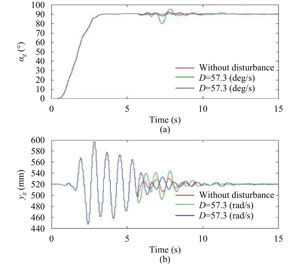
Fig. 8. Tracking performance of the predictive controller when an extra disturbance is introduced between 5.5 s to 6.5 s: (a) ag and (b) yg.
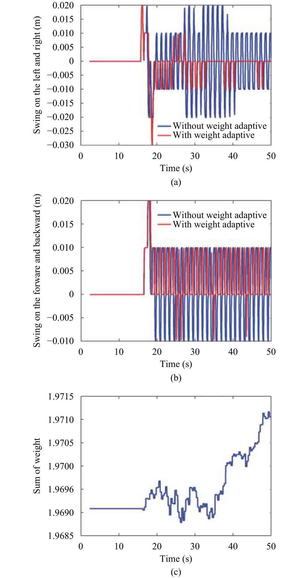
Fig. 9. Comparison and weights: (a) and (b) are comparison of swing ranges between the conventional predictive controller and the proposed adaptive predict controller, where (a) shows the movement of the payload in the left and right direction and (b) in the forward and backward direction, both are expressed in meters;(c) weights of ESN model are added up showing the trends of adaptation. The inputs to the ESN model are normalized that the weights have no units.
6. Conclusions
The control problems of modeling error and time-varying delay in anti-swing control were handled with the adaptive predictive control strategy. Importantly, a robust LED vision servo was proposed, and a tapped-delay ESN network was designed as an adaptive model to enlarge prediction horizon in the control law. Performances of the proposed scheme were verified by experimental results.
 Journal of Electronic Science and Technology2018年2期
- Journal of Electronic Science and Technology的其它文章
- Multimedia Encryption with Multiple Modes Product Cipher for Mobile Devices
- Improved Method of Contention-Based Random Access in LTE System
- Systematic Synthesis on Pathological Models of CCCII and Modified CCCII
- Secure Model to Generate Path Map for Vehicles in Unusual Road Incidents Using Association Rule Based Mining in VANET
- Mining Frequent Sets Using Fuzzy Multiple-Level Association Rules
- Improvement of an ID-Based Deniable Authentication Protocol
