Lessons learnt from a deep excavation for future application of the observational method

Raul Fuentes,Anton Pillai,Pedro Ferreira

aSchool of Civil Engineering,University of Leeds,Leeds,LS2 9JT,UK

bOve Arup and Partners,13 Fitzroy Street,London,W1T 4BQ,UK

cDepartment of Civil,Environmental&Geomatic Engineering,University College London,Chadwick Building,Gower Street,London,WC1E 6BT,UK

1.Introduction

As a design and construction framework,the observational method(OM)was introduced by Peck(1969)and has since seen many applications over the years(e.g.Glass and Powderham,1994;Powderham,1994,2002;Powderham and Rutty,1994;Peck,2001;Sakurai et al.,2003;Chapman and Green,2004;Finno and Calvello,2005;Yeow and Feltham,2008;Nicholson et al.,2014;Spross and Johansson,2017).

OM can be approached in multiple forms.However,within the context of this paper,we focus on the philosophy of EUROCODE 7(EC7)Clause 2.7(British Standards Institute,2004)to provide a framework for our discussion against an established design standard.EC7 states the following requirements for the application of the OM before construction starts:

(1)Acceptable limits of behaviour shall be established.

(2)The range of possible behaviour shall be assessed and it shall be shown that there is an acceptable probability that the actual behaviour will be within the acceptable limits.

(3)A plan of monitoring shall be devised,which will reveal whether the actual behaviour lies within the acceptable limits.The monitoring shall make this clear at a sufficiently early stage,and with sufficiently short intervals to allow contingency actions to be undertaken successfully.

(4)The response time of the instruments and the procedures for analysing the results shall be sufficiently rapid in relation to the possible evolution of the system.

(5)A plan of contingency actions shall be devised,which may be adopted if the monitoring reveals behaviour outside acceptable limits.

In particular,we will provide a commentary of the observed behaviour of a deep excavation and its impact on the first four EC7 requirements as shown above.A methodology of how to set the trigger values or a set of action plans is not covered in this article but is thoroughly presented by Spross and Johansson(2017).In this paper,the focus is on the behaviour that may affect the general application ofOM in relation to the above requirements.The commentary includes some initial guidance on how to overcome this behaviour for the future application of OM in similar conditions.

The complexity of current deep excavations,due to the congested urban environments,means that sophisticated analyses are needed to satisfy the requirements of all stakeholders involved in these projects which,in cities,also include the third-party neighbours.These analyses are typically three-dimensional(3D)numerical models that require adequate constitutive relationships to characterise soil behaviour.In the case covered in this paper,we focus on the use of the BRICK soil model(Simpson,1992),which has been validated for characteristic parameters(defined in the next section)and provides adequate design parameters for deep excavations in undrained London Clay(Ng et al.,1998;Long,2001;Yeow et al.,2006).

To date,however,a validation of most probable(also defined in the next section)BRICK soil model parameters has not yet been carried out and it is a necessity for future applications of the OM using BRICK soil model.Furthermore,it is known that excavations present 3D effects,particularly around their corners,as well as time-dependent effects that need to be considered when setting the trigger values.This is particularly necessary to avoid situations where measured movements exceed those triggers.Therefore,this paper has three main objectives:

(1)Validate a set of most probable parameters for BRICK soil model in 3D,using undrained analysis for a case study in London Clay;given that in conjunction with the already validated characteristic parameters,it can provide a sufficient range of behaviours for the application of OM.

(2)Observe the corner effects of the case study in relation to providing guidance of how these can be considered within the operation of OM.

(3)Observe the time-dependent movements and provide guidance of how these could be included in the predictions within the operation of OM.

2.Observational method-design parameters

The EC7 requirements presented above are very broad and have been approached in multiple ways by different authors.Of particular interest are the works(Prästings et al.,2014;Spross et al.,2016)applied to other types of geotechnical structures.In the context,the focus is on the design parameters and the behaviour of the retaining wall,following the recommendations of Nicholson et al.(1999).EC7 requirements 1 and 2 of the list above are related to the definition of a range of behaviours.Nicholson et al.(1999)recommended the use of two sets of design parameters to do this: ‘most probable’and ‘characteristic’.The former,with such name introduced byPowderham(1994)and Nicholson et al.(1999),defined it as:“a set of parameters that represent the probabilistic mean of all possible set of conditions.It represents,in general terms,the design condition most likely to occur in practise”.As other authors have done in the past(e.g.Yeow and Feltham,2008;Nicholson et al.,2014),we define them as those parameters that provide the closest response to reality in terms of displacements(i.e.monitoring data).The second set agrees with the terminology used in EC7(British Standards Institute,2004)and is defined as:a cautious estimate of the value affecting the occurrence of the limit state.Hence,both sets of parameters differ in their degree of cautiousness with the ‘characteristic’being a more cautious set of parameters.Both sets allow the prediction of two separate trigger values that give a range to dictate when actions are required(i.e.point 5 of the EC7 requirements).In order to fulfil EC7 requirements 3 and 4,both sets also need to provide a range of behaviours that can be easily differentiated and also monitored timely.For this,Nicholson et al.(1999)recommended that both sets of parameters are validated against real case studies using similar sites,which is what this paper provides for deep excavations.

3.Site description

3.1.Site and existing structures

The site is located in the vicinity of Aldgate Station in London,UK.The site is bounded to the southeast by St.Botolph Street,to the southwest by Houndsditch,and to the northwest by Stoney Lane(Fig.1).White Kennett Street forms the northern site boundary with the London Underground(LUL)District and Metropolitan lines running along the eastern site boundary through a cut and cover tunnel.The site dimensions are approximately 90 m×65 m(length×width).Ground level around the site rises from approximately+14 mOD to+15.5 mOD in the north/south direction,where mOD stands for metres above Ordnance Datum.

The site was occupied,before the project started,by two buildings:St.Botolph’s House and Ambassador House as shown in Fig.1.St.Botolph’s House was designed and built in the 1960s.It was an 8-storey concrete frame building on pad foundations with a single basement;the basement occupied most of the site footprint and its level was typically at+11.0 mOD.Ambassador House was built in the 1980s and occupied the northern part of the site.It was a 12-storey concrete frame building with a single basement founded on a raft.The basement was used as a car park with a ramped access off St.Botolph Street,parallel to an LUL tunnel(Fig.2).The basement level was typically at+10.5 mOD.

3.2.Adjacent structures

The LUL Circle and Metropolitan underground lines run alongside the eastern site boundary through a former open cut,which was subsequently capped in the early 1990s to form a pedestriansonly zone.A reclined retaining wall separates the LUL tunnels from the existing structure.A subway passage exists beneath St.Botolph Street and Houndsditch,to the south corner of St.Botolph’s House.The location of both structures is shown,approximately,in Fig.2,together with the footprint of the proposed building.

The new St.Botolph’s development includes demolition of the existing Ambassador House and St.Botolph’s House buildings and the construction of a new commercial of fice development.The newly built structure has fourteen storeys above two levels of basement.This means a retained height between 10.5 m and 11.5 m.

3.3.Ground investigation and conditions

The ground investigation(see Fig.2)was carried out between 4 October and 14 December 2006,using the following investigative tools:

(1)Three boreholes drilled by cable percussive methods to an average depth of 45 m below ground level;

(2)Four observation pits excavated to a maximum depth of 2.1 m to investigate areas of potential contamination;

(3)Six horizontal concrete cores to investigate existing basement walls;

(4)Six vertical cores to investigate the existing basement structure;

(5)Four inclined cores and one vertical core drilled using a Beretta T41 track mounted rotary rig to investigate the geometry and composition of the LUL reclined wall and to determine the top of the London Clay in the northern boundary of the site;

(6)Nine trial pits to locate utility services within the surrounding pavements;and

(7)Two vibrating wire piezometers and one standpipe installed in the boreholes.

This ground investigation revealed the geological sequence that was verified on site with the ‘most probable’parameters derived for each stratum presented in Table 1 as the mean of all values.Three piezometers were monitored before commencement of the works and based on these,an underdrained pro fi le(60%of the hydrostatic)was assumed for the London Clay,as shown in Fig.3.It was also assumed that the pore water pressures(PWPs)followed a hydrostatic profile for the deposits below the London Clay.

Fig.1.Site boundaries,existing adjacent buildings and existing basement levels.

3.4.Construction

3.4.1.Retaining structure

Two 1 m and 0.75 m diameter secant piled walls were installed around the perimeter as permanent works,except at the location of the cores,where 0.34 m diameter contiguous piles were used as temporary works.The smaller pile diameter of 0.75 m was selected to reduce the impact of installation on the LUL tunnels.Fig.4 shows an isometric and a plan view of the retaining wall and the location of the different wall types with their levels at the top of the capping beam and toes.It must be noted that the toe of the wall type P3 is significantly higher than the rest due to the presence of building cores requiring different construction sequences,as will be shown later.

3.4.2.Temporary works and construction sequence

The temporary works consisted of 660 mm diameter circular hollow sections(CHS)corner props mounted on 305 mm×305 mm×118 mm(length×width×height)universal columns(UCs)king posts and tie beams for all wall types,except wall type P3,where 152 mm×152 mm×30 mm(length×width×height)UC raking props connected to waling beams were used as shown in Fig.5.Details of the above sections in the UK can be found in Steel Construction Institute(2007).The propping plan can be seen in the inset of Fig.4.

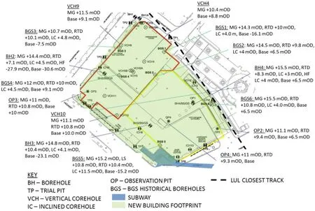
Fig.2.Location of the ground investigation points,LUL tunnel and subway locations.

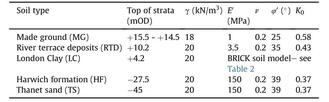
Table 1Soil stratigraphy and ‘most probable’parameters obtained from site investigation.

A bottom-up excavation sequence was adopted,as shown in Fig.6.The fi gure contains snapshots at key construction dates,starting on 5 March 2008.Prior to this date,the existing buildings were demolished,thebasementwas back filled to level+14.65 mOD,and the piles were installed for the secant piled wall.Table 3 provides a description of the main construction activities in the middle column.The modelled construction sequence in the right-hand side is based on the ‘as built’records and focussing on the north-west corner.Further details are provided in Section 4.4.

3.5.Monitoring system

3.5.1.Installed system

A comprehensive monitoring scheme was implemented on site(see Fig.7),which consisted of:

(1)37 precise levelling studs on surrounding pavements,subways,footpaths and structures.

(2)14 reflective survey targets on adjacent buildings.

(3)4 tiltmeters and 4 re fl ective survey targets for the LUL tunnel retaining wall.

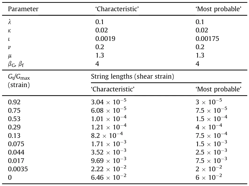
Table 2BRICK soil model parameters.

(4)8 manual inclinometers with a probe length of 0.5 m were used to take measurements within an inclinometer case embedded within the retaining wall.

(5)8 reflective survey targets on the secant piled wall capping.

3.5.2.Selection of the area of study

The area selected for close study was the north area indicated in Fig.7.This area was chosen for two main reasons:it was the only area not affected by the presence of other underground structures(i.e.LUL tunnels and the subway),which undoubtedly introduced many unknowns into the model,and secondly,both the capping beam target and inclinometer readings were available.

4.3D fi nite element model

The 3D mesh was generated using Hypermesh v.10,whereas the numerical analysis was carried out in 2010,using the LS-DYNA software(LS-DYNA,2008).The latter allows for multiprocessor analysis in parallel,which decreases computing times dramatically.A computer with a CPU Intel®Xenon®X5482@3.20 GHZ and 8.00 GB of RAM was used when the analysis was originally carried out,which led to an average computational time of approximately 25 min per stage.

4.1.Mesh and boundary conditions

Fig.8 shows general details of the mesh that was used for this project.The model height is over five times the maximum retained height,as recommended by Potts and Zdravkovic(2001).The width and breadth,inplan,are at least three times the maximum retained height as advised by Lin et al.(2003).

The model consists of 629,770 nodes,607,634 solid elements,41,286 shell elements,and 269 beam elements.These were all contained within 165 Parts(a Part is an individual entity in LSDYNA within the mesh where mainly material properties and dimensions,if appropriate,can be assigned).

Fig.9 shows the detail of the model near inclinometer Inc 06.Each colour in the figure represents a single Part as defined above.

The following displacement boundary conditions were applied to the model:(a)the horizontal base of the model was restrained in all directions;and(b)all the vertical boundaries were restrained horizontally and free to move vertically.

4.2.London Clay-BRICK soil model

All soil elements were modelled using solid elements.As shown by Grammatikopoulou et al.(2008)and Yeow and Feltham(2008),the two parameters governing the behaviour of the retaining structure,in an undrained analysis of London Clay,are the stiffness and the initial stress distribution(i.e.K0)of the soil.This agrees broadly with the findings of Whittle and Hashash(1992)and Hashash and Whittle(1996)on Boston clay and another clay of low permeability showing undrained behaviour.This means that a soil model capable of modelling the stiffness profile of London Clay as well as the initial stresses is necessary.Therefore,the BRICK constitutive soil model(Simpson,1992)was chosen;its use for deep excavations has been validated for overconsolidated clays in two-dimensional(2D)undrained analyses(Ng et al.,1998;Long,2001;Yeow et al.,2006).

Furthermore,Yeow and Feltham(2008)also showed that for multiple excavations in London Clay and the same numerical approach,a variation in London Clay parameters had a significant effect on the results.Therefore,we have used a simple elasticperfectly plastic Mohr-Coulomb soil model and the‘most probable’parameters for all the soils other than London Clay.The values are showed in Table 1.

The BRICK soil model,as first introduced by Simpson(1992),later reviewed by Pillai(1996)and lastly finalised in a 3D version which has been fully formulated by Ellison et al.(2012),was used,and it has been proven to model London Clay behaviour widely as that included by Pantelidou and Impson(2007).

Table 3Modelled and actual construction sequence.

The model’s concept is that of a man walking in a room with a series of bricks(from which the model takes its name)attached to himwith inextensible strings of different lengths.The movement of the man represents the total strain of a soil element.Plastic strains occur only when the bricks move.Each pair of string length and brick represents the maximum elastic shear strain that each proportion of soil can experience and the proportion of soil,respectively.Elastic strains are calculated as the difference between the man’s movement and the summation of all the bricks’movements weighted by the material proportion they represent.

In the analogy,when the man changes direction,some of the bricks will not move initially until the string is taut,and will swing around until they align with the new direction of movement.When one string is taut,the proportion of material represented by that brick is behaving fully plastically.Similarly,when all the bricks are moving,the whole soil is behaving completely plastically.This is how the model accounts for the phenomena described by Atkinson et al.(1990),related to changes in stiffness due to changes in strain path.

The influence of stress history,shown by Atkinson et al.(1990),due to overconsolidation,is modelled in BRICK soil model by using theβparameters;these increase the stiffness as the overconsolidation rate increases as shown by Clarke and Hird(2012)and Ellison et al.(2012).The different set of string lengths and proportion of material allows the characterisation of the stiffness S-shaped curve,using a stepwise function.The number of steps corresponds to the number of bricks and strings defined.

The relationship betweenelastic volumetric strainand the mean effective stress is very similar to that of the Cam Clay model,and uses variables analogous toλandκto characterise the virgin compression line and unloading/reloading lines,respectively.However,different to Cam Clay,BRICK soil model introduces a new parameter,ι,that provides a higher stiffness at small strains in the unloading/reloading region,by reducing the plastic strain in order to increase the elastic capacity(see Table 2).

Each couple of string and brick defines a yield surface for that particular proportion of soil.The yield function is a modified Drucker-Prager yield surface which is achieved by varying the string lengths as a function of the Lode angle in the strain space,so that the yield surface is closer to a Mohr-Coulomb hexagonal surface in the deviatoric plane in strain.The parameter used in BRICK soil model for this purpose isμ.This parameter was not originally introduced by Simpson(1992)in the BRICK soil model formulation,but later,by the same author,as the model was developed in unpublished work.

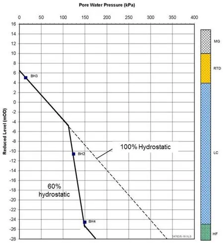
Fig.3.Measured groundwater and soil profile(please refer to Table 1 for abbreviations).

BRICK models the in situ stresses(K0)by replicating the geological history of the soil from slurry to its current state.In the London area,this means that the top of the London Clay was deposited from a slurry,later overlain by 250 m of material which was later eroded and then overlain by the current deposits;all under saturated conditions were confirmed in the study by Hight et al.(2007).Simpson(1992)presented a thorough study of the calculated profiles ofK0that justifies this approach.Other studies showing the ability of BRICK soil model to modelK0,and the general stress-strain behaviour of London Clay were presented by Ellison et al.(2012).

Two sets of parameters were used in the BRICK soil model(see Table 2): ‘Characteristic’from the originally named ‘moderately conservative parameters’in Simpson(1992)and,the ‘most probable’(to be validated in this paper)from Yeow and Feltham(2008).As it can be noticed from the table,both sets differ only in the string lengths,which results in different stiffness-strain curves,and the value ofι(i.e.the elastic stiffness in the initial region of the unloading/reloading line).The full justification is presented in Yeow and Feltham(2008),but essentially stiffness governs the problem.

Fig.4.Retaining wall model with toe and top of the capping beam levels.Inset shows the secant piled wall layout and propping arrangement at capping beam level.

4.3.Structural elements

The thicknesses and stiffness of the different elements were calculated using the following equations to ensure that the plane strain(2D)or shell(3D)elements had an equivalent bending and axial stiffness to the real structure.Hence,the thickness,t,is calculated as

whereIrealrepresents the second moment of inertia per metre of the real element,andArealshows the cross-sectional area per metre of the element.

Similarly,the stiffness is calculated as

whereErealis the Young’s modulus of the element;andAmodelis the cross-sectional area of the element in plane strainper metre,which equalst.

Since all the analyses were carried out only up tothe completion of the excavation,the short-term stiffness of the concrete,taken as 2.18 × 104MPa,was used.The steel Young’s modulus was taken as 2.1×105MPa and used to model the props.

The connections between the tubular props and retaining walls consisted of a cast-in-shoe that was fixed to the nib or retaining wall(see Fig.5)using rods in a resin filled hole.A metal plate attached to the prop was then slotted into this shoe.Rods were used to fix the prop to the shoe and, finally a grouting mix was injected between the prop and the shoe to cement it completely.Fig.5a shows the cast-in-shoe ready for prop installation on the left hand side,and a completed installation on the right.Due to this very rigid arrangement,all connections between retaining walls and temporary props were modelled as fully fixed.

The retaining walls,capping beams,slabs and other walls were modelled as shell elements;whilst the waling beams,temporary props,beams,and king posts were modelled using beam elements.

4.4.Modelling sequence

Stages 1-4 cover the site history and the construction of the existing buildings and this is critical,as explained above,to ensure that the current stress state(i.e.K0)is as accurately reproduced as possible.Stages 5-15 cover the works carried out for the construction of the new development up to the end of September2008.

Fig.10 shows the construction stages described in Table 3;each stage can be compared with the correspondent picture of the construction site,taken at the dates shown on the pictures.

5.Results and discussion

It was initially assumed that the inclinometers were fixed at the bottom:an assumption that was validated by comparison between inclinometer readings and a 2D target at the capping beam level;this will be shown later.

The horizontal movement measured by inclinometers Inc 06 and Inc 01 on or around the construction stages,de fi ned in Table 3,are shown in Figs.11 and 12,respectively.The inclinometers were installed on 22April2008and baselinereadingsobtainedon25April 2008.At the time of baseline readings,the excavation had already reached the+7.9 mOD level approximately,therefore all previous movements were lost.Fig.11 also shows that on 29 September 2008,the top of the retaining wall moved signi fi cantly towards the excavation as the temporary propping,at capping beam level,was removed.These movements should,in principle,occur very quickly.However,as they occur over time,they can be considered timedependent movements.These movements cannot be captured by an undrained analysis and will be covered later in more detail.

The effect of the ramp construction along Stoney Lane(Stage 10 in Fig.11)would have ideally been investigated through study of the movements of target No.610.However,it was obscured shortly after installation by the ramp construction itself,and later it was damaged,and therefore no results were available.An approximate effect of the construction of the ramp can be seen byexamining the behaviour of inclinometer Inc 01 in Fig.11.It shows that the installation of the ramp,after Stage 9,produces a backward movement of the inclinometer that continues up to Stage 11.The excavation of Stage 12 reverses the movement into the excavation again.In total,the ramp construction caused a backwards movement of 2 mm approximately.

The results of the FE analysis,in Fig.12,show that there is a reasonable agreement between the ‘most probable’parameters and the fi eld measurements,whereas the ‘characteristic’parameters over-predict the movements.

Fig.5.(a)Prop-wall connection details,and(b)Propping system on 21 July 2008 in the north-east corner.

Fig.13 shows the variations of the readings in target No.616,immediately adjacent to inclinometer Inc 06 and attached to the capping beam.It must be noted that,in some cases,there is a time difference of 3 d between the readings of the inclinometer and the target.This comparison validates the assumption that the inclinometer is fixed at the bottom,since inclinometer Inc 06 shows a movement of over 6 mm in Stage 15,which is close to the values shown by the 2D target around that date,within±2 mm accuracy.This figure also shows that there is a very good agreement between the FE analysis,using most probable parameters and the observed values;the FE line forms a reasonable average of the field measurements,with the difference between measured and predicted,at a given date,being around±2 mm.

Fig.6.Snapshots showing the construction sequence(DD/MM/YY).Marked in red is the FE( fi nite element)analysis area of study(date:DD/MM/YY).

Fig.7.Site map and instruments’location(dashed line indicates the FE analysis area of interest).

Fig.14 shows a comparison of vertical ground movements behind the area of study,between FE and field measurements.The FE results show a much higher settlement for point 113.This point is located behind the minipiles position(see Fig.7),and therefore,this greater settlement is probably due to theexcavation to formation level inthe vicinity of this area(see Fig.6 between 16 September 2008 and 29 September 2008).Unfortunately,point 113 was not measured on site after June 2008 and a direct comparison is not possible.

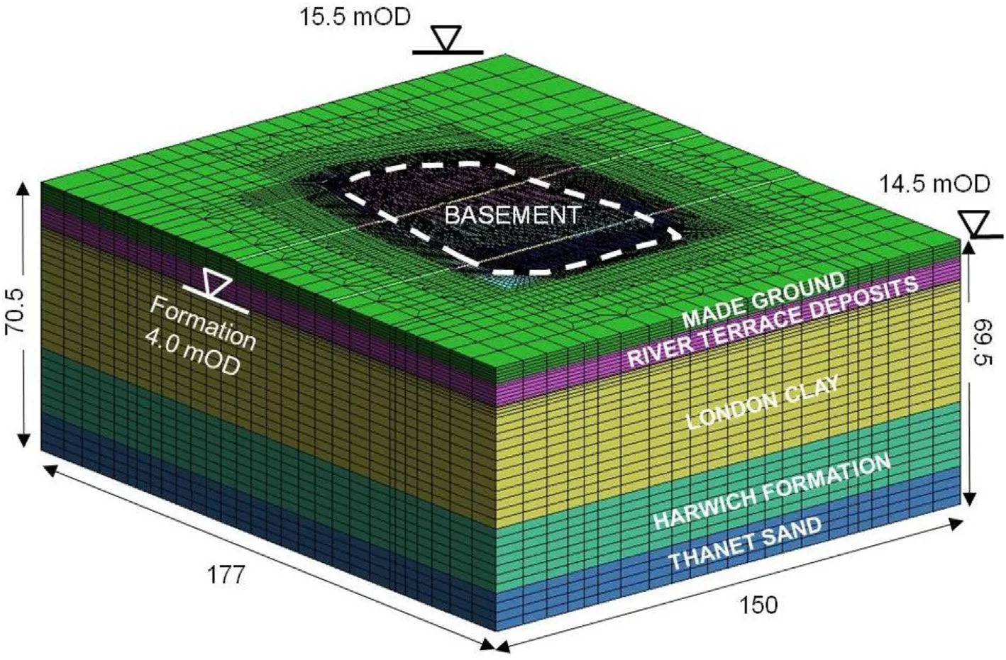
Fig.8.Mesh dimensions used in this study(unit in m).

Fig.9.FE model details in the area of interest indicating the approximate inclinometer locations(some dimensions are exaggerated).

The other fi eld measurements show that after completion of the excavation(Stage 12),there seems to be a further settlement of around 2 mm behind the retaining wall,stabilising after approximately 2 months(60 d).This is believed to be a consequence of PWP dissipation after excavation completion,which was not modelled in the numerical analysis.Richards et al.(2007)showed that PWP recovery behind a retaining wall can be very quick during excavation.The authors quoted quicker recoveries as those observed here;however,this was expected particularly since London Clay has a lower permeability than the soils covered(Richards et al.,2007).

5.1.Corner effects

Fig.14 also shows that point 112,near the corner of the excavation,shows a lower movement than point 114,which is near the centre of the wall.This indicates that the corners of the excavation have a stiffening effect,which has also been observed by other authors(St John et al.,2005;Roboski and Finno,2006;Finno et al.,2007;Fuentes and Devriendt,2010;Hashash et al.,2011;Hong et al.,2015).

Fig.15 plots the ratio of movements between the points 112 and 114,together with the results from the FE analysis using the‘mostprobable’parameters.The field measurementsshow negative values and great variability.This is more apparent at early stages of the project,when most of the enabling construction works took place,which can be explained by interferences from the enabling works on site during this time.The trend seems to be much clearer at the later stages of the excavation after the maximum excavation level is reached,and the ratio remains relatively constant.

A comparison can be carried out by using a value of 67%as suggested by Fuentes and Devriendt(2010)or using Eq.(3)from Roboski and Finno(2006),as shown in Fig.15:

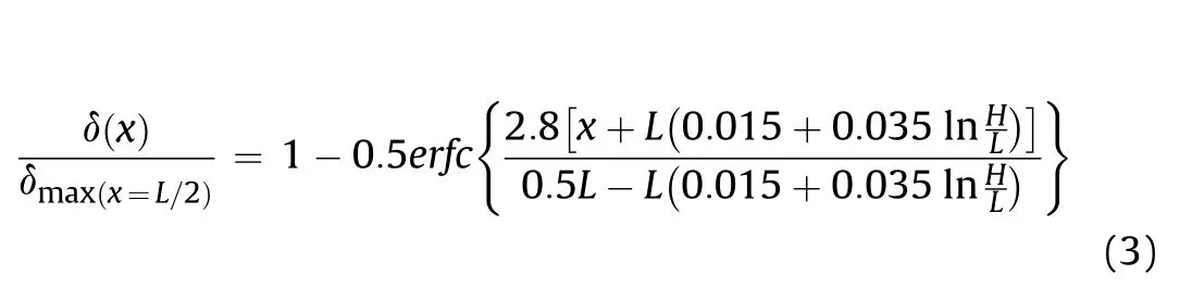
Fig.10.Modelled construction sequence in LS-DYNA-comparison of Table 3 and Fig.6(date:DD/MM/YY).

wherexis the distance from the wall corner,δ（x）is the lateral displacementof the points along thewall length,inplan,andδmaxis the lateral displacement at the middle of the retaining wall,also in plan;anderfc(·)is the error function.

Eq.(3)hence expresses the ratio δ(x)/δmaxversusL/H.Fig.16 plots this equation for the case of the corner wherex=0,hence allowing calculation of the ratio δcorner/δmax.The fi tted exponential line in the fi gure(written in Eq.(4))has a coef fi cient of determination(R2)close to 1,and constitutes an interesting estimation tool for engineers to consider the importance of corner effects for particular excavation geometry:

In order to test Eq.(4),we applied it to the case study presented in this paper,whereLis 90 m andHis 11.5 m.This results in a value ofδcorner/δmaxequal to 34.2%,plotted in Fig.15.This value shows a better agreement to the field data than that(67%)of Fuentes and Devriendt(2010),which nonetheless represents a reasonable upper-bound value to the data.

5.2.Time-dependent movements

As mentioned above,time-dependent movements are apparent in the wall.Fig.17 shows both the movement experienced at the wall,and its rate of change,after prop removal for all the available inclinometers as shown in Fig.7.The rate of movement was calculated as the change in movement between readings,divided by the number of days between them.Both graphs show that after approximately 160 d,when around 9 mm of movement occurs at the top of the wall,the rate of movement is negligible.Before stability is reached,the rate of movement ranges between+0.5 mm/d and-0.5 mm/d,with the exception of some outliers that can only be explained by rogue readings as subsequent measurements of the same instrument returned to the normal bounds.Furthermore,a literature search,presented in Table 4,shows that the maximum reported values of time-dependent movements are 1.07 mm/d,and for soil conditions it is more prone to such movements than those presented in this case study.It is therefore concluded that these “rogue”values are most likely a consequence of individual inaccurate readings.

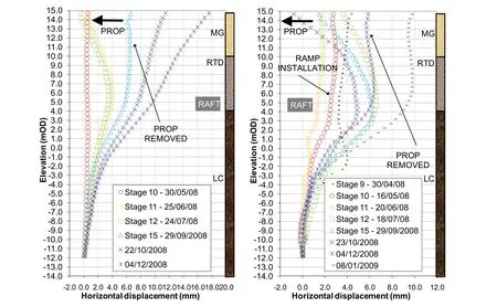
Fig.11.Inclinometer readings-Inc 06(left)and Inc 01(right).LC:London Clay;RTD:River Terrace Deposits;MG:Made ground.Date:DD/MM/YY.

Fig.12.Comparison between inclinometer Inc 06 readings and FE analysis:(a)using ‘most probable’,and(b)using ‘characteristic’parameters.

The origins of these movements are very difficult to decipher,with some authors attributing it to soil creep,consolidation and/or relaxation(Roscoe and Twine,2010).Without accurate PWP measurements,it is impossible to separate them.It is clear that more case studies that provide enough evidence are needed before reaching the final conclusions about these movements.The limited case studies available,however,seem to indicate that consolidation dominates these types of movements,not creep.For example,Liu et al.(2005)showed through accurate PWP readings that the time-dependent movements attributing to soil creep were very small.A similar result was presented by Richards et al.(2007)who justified the timedependent movements through consolidation theory.Finno et al.(2002)showed this for ground movements,not wall displacements,although they also attributed part of the time-dependent movements to creep.This shows the difficulty of the problem.

Fig.13.Horizontal displacement of target No.616 at the same location of the inclinometer Inc 06 and FE results.Positive movement indicates movement towards the excavation.The average line was calculated in Excel with a period of 6 d.

Fig.14.Results comparison between FE analysis and levelling readings.

6.Implications to the observational method

The implications of the findings of this paper compared to the EC7 requirements shown at the outset are displayed below.The use of the most probable parameters and characteristic in BRICK soil model has been demonstrated to provide both a realistic and cautious representation of the behaviour of this excavation,which complies with the EC7 requirement of“acceptable limits of behaviour shall be established”.For example,the results for selected stages are shown in Table 5 and can be used as the trigger values in terms of the maximum acceptable deformation which,as mentioned previously,is of widespread use in retaining walls.

On the other hand,the demonstrated corner effects show that unless they are considered,significant over-designs and mitigation measures could be unduly set in place.It is noted that the distribution in Fig.16 is exponential.This means that for all excavations with values ofL/Hequal to or greater than 1.5,the ground movements at the corner will be overestimated.For example withL/H=1.5,the over-estimate is a factor of 2.Similarly,for a value ofL/H,like 18,this overestimate will be 3.3 times.It should be noted that most excavations will be within these ranges of 1.5＜L/H＜18.

Equally,the time-dependent movements may have a significant effect on this EC7 criterion.For example,based on the observed information and literature review,it is concluded that a rate of movement of 0.5 mm/d can be expected for excavations of this type built in London Clay.Knowing this rate allows comparing the current displacement to the trigger value,giving an indication of how long it will take to reach the trigger value.This can be written as

Fig.15.Ratio of vertical ground movements behind the retaining wall,between the corner(settlement monitoring point 112)and the centre(settlement monitoring point 114)approximately-not showing calculated values for clarity.

Fig.16.Ratio ofδcorner/δmaxfor different values of L/H based on Roboski and Finno(2006),together with an exponential fi t to the data points.

where δTand δCare the trigger and the current displacements,respectively;and˙δis the time-dependent displacement ratio(0.5 mm/d for our case).Fis a factor and the designer can use to ensure that,when an excavation is left idle for a timetlapsed,the trigger valueδTwill not be reached as will be shown later.

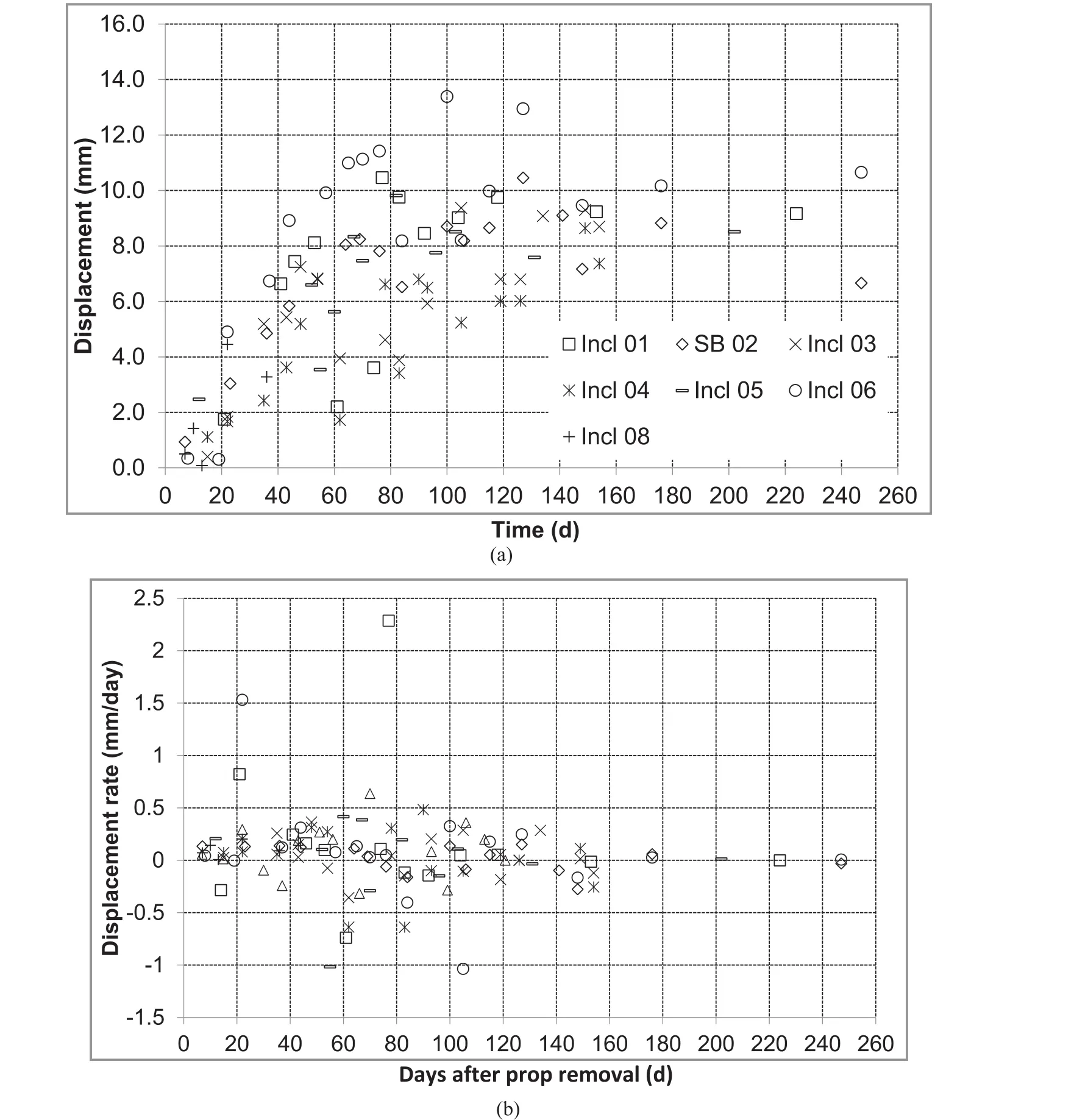
Fig.17.Observed change in movement at the top of the wall from the day of prop removal-total movement in mm(a)and rate of movement rate in mm/d(b).

Eq.(5)can also be used to compare two different sets of trigger values to ensure that a practicable range is provided to cater for the displacement rate.In this case,we use the example of most probable and characteristic triggers,but this would work equally for any two different trigger values.Hence,Eq.(5)can be rewritten as

where δMPand δCHare the most probable and characteristic trigger values,respectively.Eqs.(5)and(6)should be another consideration when defining both sets of the design parameters and the trigger values in the context of displacement rates(time-dependent movements).

For example,for the values of Table 5 in Stage 15 and a value ofF=1,the time lapsed for a movementδMP=7.09 mm to reach δCH=15.9 mm would be 17.62 d,which is adequate for monitoring purposes and to identify and measure trends.However,in other circumstances when small displacements are presented,both trigger values may not provide enough distance in the presence of time-dependent movements.For example at Stage12 in Table 5,the trigger values mean that only 5.2 d would lapse for a wall at the deformation established using the most probable parameters to reach the deformation calculated using the characteristic parameters.This reinforces the relevance of these time-dependent movements as 5.2 d may not be deemed sufficient to enact any actions or even to monitor with sufficient frequency.Designers must be aware of this,which is particularly applicable for the cases of small displacements.Although the development of a full set of guidelines to cater for this is outside the scope of this paper,we present the potential use of the factorF.This essentially allows redefining a trigger value to provide sufficient distance,if that is the appropriate solution,to cater for time-dependent movements.An example is provided below.

Table 4Database of the time-dependent movements.

Table 5Wall displacement at different stages.

Fig.18 shows a plot of the value ofFfor the case of Stage 15 in Eq.(6)using the ‘most probable’and ‘characteristic’parameters and˙δ=0.5 mm/d.Values ofFgreater than 1 mean that the trigger value will be reached faster,and the converse occurs for values lower than 1.In other words,in this example,using a value ofF=0.58 means that the lapsed time is 40 d as opposed to 17.62 d as previously calculated forF=1.If a decision was made that 40 d were required,e.g.imposed due to construction delays usingF=0.58 would mean increasing the‘characteristic’value to 27.09 mm from 15.9 mm.This artificial increase of the‘characteristic’trigger value would,naturally,need to be compared against the limit state of the structure to satisfy the designer.

An additional consequence of the above is that the monitoring system needs to be capable of measuring deformation with enough frequency to capture information at the rate dictated by˙δ.This is to comply with EC7 requirements that“a plan of monitoring shall be devised,which will reveal whether the actual behaviour lies within the acceptable limits.The monitoring shall make this clear at a sufficiently early stage,and with sufficiently short intervals to allow contingencyactions to be undertaken successfully”and “the response time of the instruments and the procedures for analysing the results shall be sufficiently rapid in relation to the possible evolution of the system”.

For example,using Eq.(5),assumingF=1,and a requirement to have four measurements between the current displacement value and the trigger value that should be compared,the required frequency of readings can be calculated as

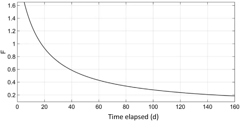
Fig.18.Values of F versus tlapsed.

Eq.(7)shows that for˙δ=0.5 mm/d,the frequency of readings is twice the distance,in mm,between trigger and current values.In this case,we used four readings between the values for illustration purposes but the others can be used according to the needs on a case by case basis.For the example of Stage 14 using the most probable and characteristic values,to have four readings would mean that a frequency of readings of 1.3 d(almost every day)was required over the 5.26 d that it would take to reach characteristic value.

Hence,Eq.(7)can be used at any stage of excavation to compare the current displacement versus the trigger value to understand the frequency of readings needed for a certain number of total readings when time-dependant movements are presented.

In summary,we suggest that,when an undrained analysis is carried out,the trigger values will need to be defined to reduce the probability of reaching a limit state(i.e.complying with EC7 second requirement of“the range of possible behaviour shall be assessed and it shall be shown that there is an acceptable probability that the actual behaviour will be within the acceptable limits”).This will provide a sufficient range to allow adequate monitoring and actions due to time-dependent movements occurring.

7.Conclusions

A comprehensive case study of a deep excavation in an overconsolidated clay has been introduced.The analysis of the data highlighted the main observations listed below:

(1)The BRICK soil model using the ‘most probable’parameters gave good predictions of wall movement and reasonable ground movements when compared to the instrumentation readings.In combination with the previously validated‘characteristic’parameters,both offer acceptable limits of behaviour and provide an adequate range,therefore validating the new set of parameters for an excavation in London Clay and its future application under the OM.This complies with EC7 requirements 1 and 2.

(2)Corner effects are important when considering the application of the OM,in particular when establishing the trigger values derived from 2D FE analysis.Assuming a unique value of deformation for the entire length of the wall,in plan,is over-cautious nearer the corners.This is more relevant in relatively long excavations-e.g.high values ofL/H-where savings could be made towards the corners through careful consideration of corner effects.

(3)Time-dependent movements are observed in retaining walls.These stabilise after approximately 160 d when approximately movement of 9 mm has occurred.At this time,the rate of movement is negligible but,according to the data,it rangesbetween+0.5 mm/d and-0.5 mm/d.This agrees with other results shown in the literature.

(4)A simple undrained analysis,using an advanced soil model,predicts the behaviour of the retaining wall and ground realistically,until the above time-dependent movements start to occur.This means that even for relatively fast moving construction projects,an undrained analysis using most probable parameters may under-predict wall movements and ground settlement when the site is left idle following the removal of a prop.This has important implications in the application of the OM which relies heavily on accuratea prioridefinitions of trigger values.

(5)It is therefore recommended that,should an undrained

analysis be carried out,an additional movement rate should be added to the predicted movements to account for the above and prevent unwarranted breaches of trigger values.(6)This case study and others in the literature seem to indicate that a value of 0.5 mm/d is a reasonable upper-bound value to use for a wide range of soil types,construction sequences and excavation depths.However,care must be exercised when defining rates of movement and duration when defining the trigger values.

(7)Based on all of the above observations in this case study,we

have presented a methodology to consider these timedependent movements both in the definition of trigger values and frequency of readings in line with the EC7 requirements as shown above.

Conflicts of interest

We wish to confirm that there are no known conflicts of interest associated with this publication and there has been no significant financial support for this work that could have influenced its outcome.

Acknowledgments

The authors would like to acknowledge the EPSRC for their funding to undertake this research.Equally we would like to thank Martha Salamanca from Arup for her comments on the manuscript and help writing it.

Atkinson JH,Richardson D,Stallebrass SE.Effect of recent stress history on the stiffness of overconsolidated soil.Géotechnique 1990;40(4):531-40.

British Standards Institute.Geotechnical design Part 1:General rules.Eurocode 7:Geotechnical design-Part 1:General Rules.2004.

Chapman T,Green G.Observational method looks set to cut city building costs.Proceedings ofthe Institution ofCivilEngineers -CivilEngineering 2004;157(3):125-33.

Clarke SD,Hird CC.Modelling of viscous effects in natural clays.Canadian Geotechnical Journal 2012;49(2):129-40.

Ellison KC,Soga K,Simpson B.A strain space soil model with evolving stiffness anisotropy.Géotechnique 2012;62(7):627-41.

Finno RJ,Bryson S,Calvello M.Performance of a stiff support system in soft clay.Journal of Geotechnical and Geoenvironmental Engineering 2002;128(8):660-71.

Finno RJ,Calvello M.Supported excavations:observational method and inverse modeling.Journal of Geotechnical and Geoenvironmental Engineering 2005;131(7):826-36.

Finno RJ,Blackburn JT,Roboski JF.Three-dimensional effects for supported excavations in clay.Journal of Geotechnical and Geoenvironmental Engineering 2007;133(1):30-6.

FuentesR,DevriendtM.Ground movements around corners of excavations:empirical calculation method.Journal of Geotechnical and Geoenvironmental Engineering 2010;136(10).https://doi.org/10.1061/(ASCE)GT.1943-5606.0000347.

Glass PR,Powderham AJ.Application of the observational method at the limehouse link.Géotechnique 1994;44(4):665-79.

Grammatikopoulou A,St John HD,Potts DM.Non-linear and linear models in design of retaining walls.Proceedings of the Institution of Civil Engineers-Geotechnical Engineering 2008;161(6):311-23.

Hashash YMA,Whittle AJ.Ground movement prediction for deep excavations in soft clay.Journal of Geotechnical Engineering 1996;122(6):474-86.

Hashash YMA,Song H,Osouli A.Three-dimensional inverse analyses of a deep excavation in Chicago clays.International Journal for Numerical and Analytical Methods in Geomechanics 2011;35(9):1059-75.

Hight DW,Gasparre A,Nishimura S,Minh NA,Jardine RJ,Coop MR.Characteristics of the London clay from the terminal 5 site at heathrow airport.Géotechnique 2007;57(1):3-18.

Hong Y,Ng CWW,Liu GB,Liu T.Three-dimensional deformation behaviour of a multi-propped excavation at a ‘green field’site at Shanghai soft clay.Tunnelling and Underground Space Technology 2015;45:249-59.

Hsiung BCB.A case study on the behaviour of a deep excavation in sand.Computers and Geotechnics 2009;36(4):665-75.

Kung GTC.Comparison of excavation-induced wall deflection using top-down and bottom-up construction methods in Taipei silty clay.Computers and Geotechnics 2009;36(3):373-85.

Lin DG,Chung TC,Phien-Wej N.Quantitative evaluation of corner effect on deformation behaviour of multi-strutted deep excavation in Bangkok subsoil.Journal of the Southeast Asian Geotechnical Society 2003;34(1):41-57.

Lin HD,Ou CY,Wang CC.Time-dependent displacement of diaphragm wall induced by soil creep.Journal of the Chinese Institute of Engineers 2002;25(2):223-31.

Liu GB,Ng CWW,Wang ZW.Observed performance of a deep multistrutted excavation in Shanghai soft clays.Journal of Geotechnical and Geoenvironmental Engineering 2005;131(8):1004-13.

Long M.A case history of a deep basement in London Clay.Computers and Geotechnics 2001;28(6-7):397-423.

LS-DYNA.Civil engineering application program.2008.Oasys Limited,Livermore Software Technology Corporation,Version 940.

Ng CW,Simpson B,Lings ML,Nash D.Numerical analysis of a multipropped excavation in stiff clay.Canadian Geotechnical Journal 1998;35(1):115-30.

Nicholson D,Tse CM,Penny C.The observational method in ground engineering:principles and applicationsvol.185.CIRIA;1999.

Nicholson D,Yeow HC,Black M,Glass P,Man CL,Ringer A.Application of observational method at crossrail tottenham court road station,UK.Proceedings of the Institution of Civil Engineers-Geotechnical Engineering 2014;167(2):182-93.

Ou CY,Lai CH.Finite-element analysis of deep excavation in layered sandy and clayey soil deposits.Canadian Geotechnical Journal 1994;31(2):204-14.

Ou CY,Liao JT,Cheng WL.Building response and ground movements induced by a deep excavation.Géotechnique 2000;50(3):209-20.

Pantelidou H,Impson BS.Geotechnical variation of London clay across central London.Géotechnique 2007;57(1):101-12.

Peck RB.Advantages and limitations of the observational method in applied soil mechanics.Géotechnique 1969;19(2):171-87.

Peck RB.The observational method can be simple.Proceedings of the Institution of Civil Engineers-Geotechnical Engineering 2001;149(2):71-4.

Pillai A.Review of the BRICK model of soil behaviour.Imperial College London;1996.

Potts DM,Zdravkovic L.Finite element analysis in geotechnical engineering:volume two-Application.Thomas Telford Publishing;2001.

Powderham AJ.An overview of the observational method:development in cut and cover and bored tunnelling projects.Géotechnique 1994;44(4):619-36.

Powderham AJ,Rutty P.The observational method in value engineering.In:Proceedings of 5 th international conference&exhibition on piling and deep foundations.Bruges,Belgium:Deep Foundations Institute;1994.

Powderham AJ.The observational method-learning from projects.Proceedings of the Institution of Civil Engineers-Geotechnical Engineering 2002;115(1):59-69.

Prästings A,Müller R,Larsson S.The observational method applied to a high embankment founded on sulphide clay.Engineering Geology 2014;181:112-23.

Richards DJ,Powrie W,Roscoe H,Clark J.Pore water pressure and horizontal stress changes measured during construction of a contiguous bored pile multipropped retaining wall in Lower Cretaceous clays.Géotechnique 2007;57(2):197-205.

Roboski J,Finno RJ.Distributions of ground movements parallel to deep excavations in clay.Canadian Geotechnical Journal 2006;43(1):43-58.

Roscoe H,Twine D.Design and performance of retaining walls.Proceedings of the Institution of Civil Engineers-Geotechnical Engineering 2010;163(5):279-90.Sakurai S,Akutagawa S,Takeuchi K,Shinji M,Shimizu N.Back analysis for tunnel engineering as a modern observational method.Tunnelling and Underground Space Technology 2003;18(2-3):185-96.

Simpson B.Retaining structures:displacementand design.Géotechnique 1992;42(4):541-76.

Spross J,Johansson F.When is the observational method in geotechnical engineering favourable?Structural Safety 2017;66:17-26.

Spross J,Johansson F,Uotinen LKT,Ra fiJY.Using observational method to manage safety aspects of remedial grouting of concrete dam foundations.Geotechnical and Geological Engineering 2016;34(5):1613-30.

St John HD,Zdravkovic L,Potts DM.Modelling of a 3D excavation in finite element analysis.Géotechnique 2005;55(7):497-513.

Steel Construction Institute.Steelwork design guide to BS 5950-1:2000.Vol.1,Section properties,member capacities.2007.Steel Construction Institute.

Whittle AJ,Hashash YMA.Analysis of the behaviour of propped diaphragm walls in a deep clay deposit.In:Retaining structures,proceedings of the conference.Cambridge,UK:Thomas Telford Publishing;1992.p.131-9.

Yeow HC,Nicholson DP,Simpson B.Comparison and feasibility of three dimensional finite element modelling of deep excavations using non-linear soil models.In:Numerical modelling of construction processes in geotechnical engineering for urban environment.CRC Press;2006.p.29-34.

Yeow H,Feltham I.Case histories back analyses for the application of the observational method under Eurocodes for the Scout project.In:The 6th international conference on case histories in geotechnical engineering.Arlington,VA,USA:Missouri University of Science and Technology;2008.p.1-13.