Modeling and identification for soft sensor systems based on the separation of multi-dynamic and static characteristics☆

Pengfei Cao *,Xionglin Luo ,Xiaohong Song

1 College of Electrical Engineering and Automation,Shandong University of Science and Technology,Qingdao 266590,China

2 Research Institute of Automation,China University of Petroleum,Beijing 102249,China

3 State Grid Shandong Electric Power Company Zibo Power Supply Company,Zibo 255000,China

1.Introduction

Over the last two decades,soft sensor technique hasbeen extensively studied and increasingly implemented in industrial processes.It solves the real-time measurement problem for important quality variables,and these variables indicate the production quality directly and play an indispensable role in process control[1–3].The soft sensor model,which is built based on massive amounts of measurements of quality and easily measured variables(primary and secondary variables),is the core of this technique[4,5].In our last contribution,a new type of soft sensor model consisting of a dynamic sub model in cascade with a static one has been proposed[6,7].And it could be named as the separation of dynamic and static characteristics based model(or characteristics-separation-based model in brief).Dynamic and static sub models build the dynamic and static relationships between primary and secondary variables respectively.The dynamic and static characteristics are described sufficiently based on these two models,and the parameters have physical interpretation and offer effective information for process control and optimization.

However,there exist two main limitations in the last research[6,7]:(1)the time constant,i.e.the dynamic sub model parameter,is designated as the same for multi-input soft sensor systems;(2)the identification is conducted in the single-rate case,and the improved stochastic Newton recursive(SNR)algorithm is applicable at this moment.Actually,the time constant of the dynamic process between the primary variable and a certain secondary variable is likely to differ from those of other processes.Therefore,one contribution in this paper is that the multidynamic characteristics of the soft sensor systems have been considered in the model with multi-time-constant.

As is well known,soft sensor systems exhibit dual-rate characteristics with slow sampled primary variable and fast sampled secondary variables[8–10].So,the recursive algorithm in our last contribution cannot be directly used for actual system.To solve the dual-rate system identification,Ding and Chen proposed one effective method that directly estimates the parameters of the single-rate model with an auxiliary model[11–13].The basic idea of the auxiliary-model-based approach is to replace the unmeasurable variable with the estimated values.The consistency of the algorithm for time-invariant systems has been proven[11,14].This method is also adopted in this study.However,the estimated values of the quality variable from the conventional auxiliary model(termed as primary auxiliary model in Section 4)may be divergent,which prevents the recursion process.To overcome the problem,another nonlinear auxiliary model(termed as secondary auxiliary model in Section 4)is first presented to cooperate with the primary one to provide the estimated values for next recursion.These two auxiliary models work in specific switching mechanism.The double-auxiliary model based stochastic Newton recursive(DAM-SNR)algorithm is then derived and utilized for the identification of the proposed soft sensor model together with the SNR algorithm.

The rest of this paper is organized as follows.In Section 2,the characteristics-separation-based model with multi-time-constant is given.In Section 3,the sub step identification way is illustrated.Section 4 gives the SNR algorithm,and shows the structure and feature of DAM-SNR algorithm.The identification procedure for soft sensor model is specified in detail in Section 5.The p H neutralization process is employed to demonstrate the effectiveness of the soft sensor model and the algorithms in Section 6.The final remarks are made in Section 7.

2.Characteristics-Separation-Based Model with Multi-Time-Constant

2.1.The previous model

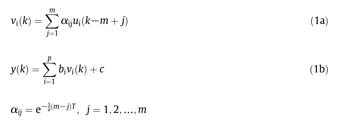
In our last study[6,7],we have derived the following discrete model for multi-input and single-output(MISO)soft sensor system:

{ui,i=1,2,…,p}and y represent the secondary and primary variables respectively,and{vi}represents the intermediate variable;a represents the time constant,and m refers to the number of historical data of each secondary variable with the same value[6];k and k−m+j indicate sampling time;{αj,j=1,2,…,m}is the dynamic weight;{bi}and c are the static model parameters.Eq.(1a)and(1b)represent the dynamic and static sub models.The dynamic relationship between the secondary and intermediate variables is built based on the dynamic sub model,which is equal to the one between secondary and primary variables with unit gain.The static relationship between primary and intermediate variables is built based on the static sub model,which is equal to the one between secondary and primary variables.We can write Eq.(1a)and(1b)as

In the above equation,it is easy to see that the dynamic model parameters multiply the static ones.The model parameters would alter with working condition changing.With changing parameters,the linear model exhibits time-varying characteristics and is utilized to approximate the real soft sensor system.The nonlinear characteristics of the system will be reflected in this way.Thus,the Eq.(1a)and(1b)actually shows the nonlinear and dynamic characteristics of soft sensor systems.

In fact,the model(Eq.(1a)and(1b))could be rewritten into a more general form as where numerous model types,such as ANN,SVM,et al.,could be adopted for f(•).And the weights in the first part of Eq.(2)may be fixed or changed.The similar research achievements about this type of model(Eq.(2))have been reported in several manuscripts[15–17].Generally,industrial process is conducted in some steady state working condition and the soft sensor systems are basically stable,therefore,linear model(Eq.(1b))is enough for f(•)in applications.On the other hand,adopting linear model could reduce modeling complexity and make the model easy to operate and update online.In this study,the general model(Eq.(2))would not be discussed further.

2.2.The improved model

One of the main limitations of the model(Eq.(1a)and(1b))is that only one time constant is considered.Actually,the response speed of the primary variable with one secondary variable changing may differ from others considerably.The soft sensor system has multi-dynamic characteristics,and it is necessary to consider various time constants in the model.To describe soft sensor system more accurately,we could write the dynamic relationship under some working condition as

Let

and we have

Transforming Eq.(4a)and(4b)into the time-domain model,we have

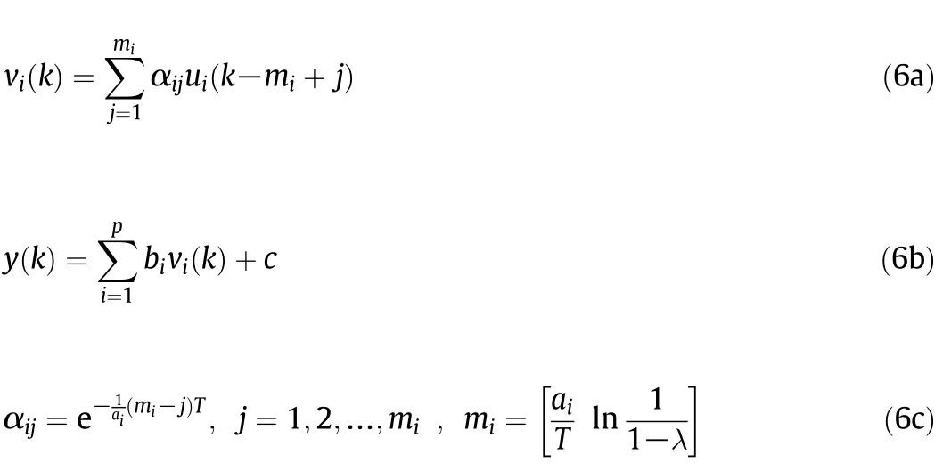
Finally,we obtain the soft sensor model as

λ represents the permissible error limit,and[·]represents the first integer greater than itself[6];T is the fast sampling period for secondary variables.

3.Substep Identification Mode

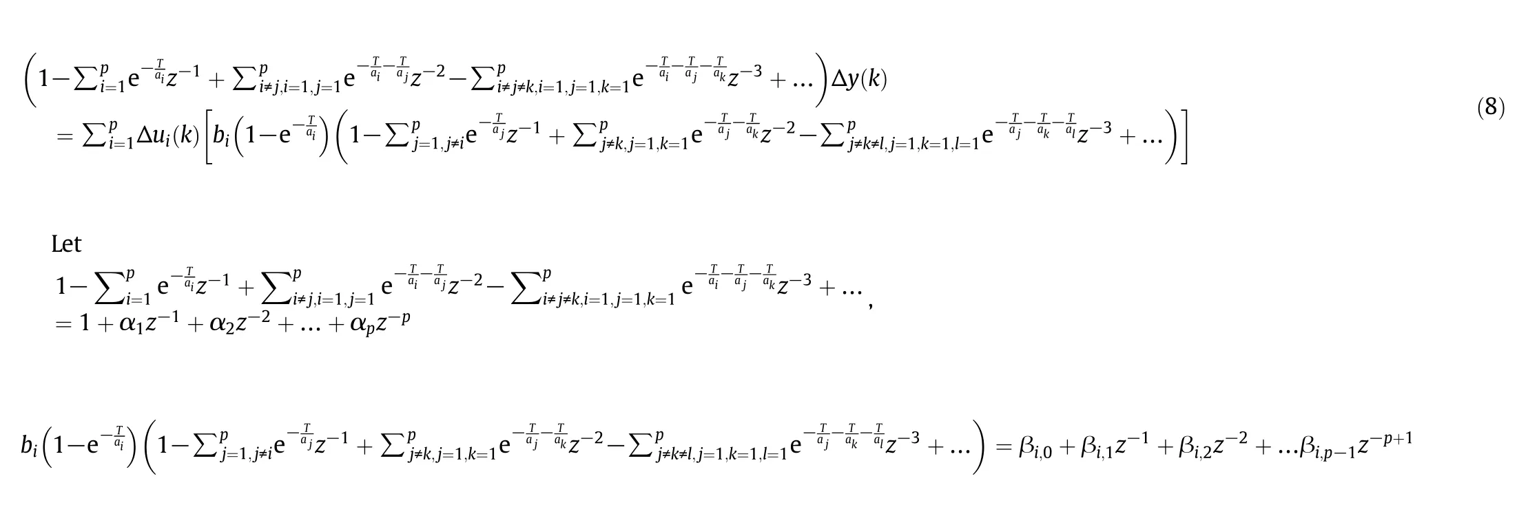
We do not identify the soft sensor model(Eq.(6a)and(6b))directly,but the corresponding models instead following the substep way.Discretize Eq.(3),and we have

where z represents the forward shift operator and z−1x(k)=x(k− 1).Then

Multiplying both sides of Eq.(8)by 1−z−1,we have

Finally,we obtain

After identifying Eq.(10),we have the estimation

Then,it is easy to obtain the estimations for intermediate variable{vi}according to Eq.(6a),(6c).With{vi}and the measurements of the primary variable,the static model parameters would be obtained through the identification of Eq.(6b).

The substep identification mode is summarized as follows:identify the model of Eq.(10) first and then the one of Eq.(6b).There are several reasons for choosing substep mode: first,it has been discussed that the soft sensor model parameters have some physical significance and may give us some guidance for process control,however,these model parameters are multiplied together(Eq.(6a)and(6b)),and it may not be able to obtain their accurate estimations with conventional optimization approaches;secondly,substep way makes it more flexible to update the proposed model online,such aschanging the dynamic model parameters only within comparatively short time and the static model parameters after long period,or in other manners,and such practice could also reduce the calculation online.

It may be doubted that Eq.(10)exhibits the relationship between the secondary and primary variables,and why it cannot be used as the soft sensor model.The reasons are as follows.Firstly,it has been explained that the model parameters in Eq.(6a)and(6b)have some physical significance and it's necessary to obtain them to make some guidance for process control and optimization.Secondly,the number of the parameters of Eq.(10)is p×(p+1),which is p times the number of the ones in Eq.(6b);however,for convenience in application,the dynamic and static sub models are updated in different rates,and the static submodel which exhibits the steady-state relationship of the system is usually updated with relatively faster frequency.

4.Introduction to the Recursive Algorithms

In this section,two recursive algorithms are given:the SNR and the DAM-SNR algorithms.At each slow-sampling period,the proposed model would be updated based on them.

4.1.The SNR algorithm

This algorithm is based on gradient-descent ideas and employs sample covariance matrix to control the update directions.Its description involves two updaterelations:one for the update of the weight estimate and the other for the update of the sample covariance matrix[18,19].We have the recursive algorithm as follows:

whereand R(k)represent the parameter estimation and sample covariance matrix;{ρ(k)}is the forgetting factor;φ(k)is defined as the information vector;z(k)is the output variable,and indicates y(k)for the models in Eqs.(10)and(6b).Given the dual-rate characteristics of the soft sensor systems,assume the slow sampling period for primary variable as qT(q is supposed as an integer and q＞1).q is defined as the sampling period ratio.Then,we could rewrite Eq.(12)into

At each slow sampling period,the parameter estimations would be updated.It should be noticed that the values of{ρ(kq)}depend on specific situation,such as to satisfy Eq.(13)in reference[6]for time invariant system,or be some constant for time-varying system[6].

4.2.The DAM-SNR algorithm

For Eq.(10),we have

and for Eq.(6b)we have

As soon as we obtain the estimation for(Eq.(11)),the intermediate variable will be easily calculated based on Eq.(6a).And then,{φ2(kq)}would be obtained.Therefore,the model identification for Eq.(6b)could follow the algorithm in Eq.(13)absolutely.However,the primary variable is sampled every other qT,and we do not have the inter samples{y(kq+i),i=1,2,…,q − 1}.Thus,{φ1(kq)}cannot be obtained at each recursion.To overcome the problem,auxiliary model technique is utilized to substitute the inter samples with their estimations.From Eq.(10),we have the auxiliary model as

Eq.(15)is defined as primary auxiliary model,^ϕ1(kq−i)represents the information vector estimation.

In general,soft sensor systems are stable and there have the time constantsHowever,during the recursion process,it may appear that the above conditions do not satisfy.The estimations from Eq.(15)would diverge,especially for the case of large sampling period ratio,and the recursion will cease at this time.This may also happen for other algorithms based on auxiliary model.Therefore,a secondary auxiliary model is first proposed to assist providing inter sample estimations,and it could be expressed in an abstract form as

N(•)refers to some nonlinear model,which is built based on the measured data{y(kq),u1(kq),u2(kq),…,up(kq)}.

These two auxiliary models work in a switching mechanism:the information vector estimation is provided mainly by primary auxiliary model(Eq.(15));when the inter sample estimations appear divergent,the secondary one(Eq.(16))functions.

Finally,the following DAM-SNR algorithm will be adopted for the identification of Eq.(10):

And the switching mechanism is shown in Fig.1.

For this algorithm,there are several remarks to illustrate:

(1)The main purpose of adopting secondary auxiliary model is to guarantee the identification for Eq.(10).There are several reasons for choosing nonlinear model: first,Khargonekar pointed out that the samples at the slow sampling period exhibited periodically time-varying characteristics,and this characteristic could be embodied by some nonlinear model which was built with the slow sampled data[20];secondly,there have been many researches on nonlinear models for soft sensor systems and successful applications[17,21-23].Even so,it could not be substituted for the proposed model,and the explanation could refer to[6,7].

(2)The secondary auxiliary model only works when the inters ample estimations diverge.The reliability of the inter sample estimations from the primary auxiliary model is consolidated when the model parameters approach to the true values,and promotes the convergence of the parameters in turn.Therefore,the secondary auxiliary model may not provide the inters ample estimations alone and only acts as necessary.On the other hand,the divergent phenomenon generally appears at the preliminary stage of the recursion process.In most cases,just the primary auxiliary model works,and this will be shown in the case study.

(3)When the inter sample estimations appear divergent,the previous parameter estimations could not be used to provide in formation vector estimations.If so,the recursion is more likely to cease with this parameter estimations.

(4)We give the judgment criteria for the divergent phenomenon:set a threshold δ for primary variable according to actual situation;if the inters ample estimation from the primary auxiliary model keeps on exceeding to the threshold,the estimations are regarded to be divergent.

5.Identification Procedure

We have the identification procedure for the proposed soft sensor model:

(1)Select one type of nonlinear model and train it off-line based on sufficient measurements{y(kq),u1(kq),u2(kq),…,up(kq),k=1,2,…}.Then,we obtain the secondary auxiliary model N(•).

(2)Initializefor the identification of Eq.(10);setfor the identification of Eq.(6b).Here,ε1and ε2are sufficiently small positive real vectors;γ1and γ2are sufficiently large real numbers.

(3)For Eq.(10),make useto estimate the inter samples before kq.If the inter sample estimations are bounded,use the primary auxiliary model to provide;otherwise,adopt N(•).Update the model parameters of Eq.(10)based on the algorithm of Eq.(17)and obtain the estimation forbased on Eq.(11).The estimations of{vi(kq)}will be obtained by Eq.(6a).

(4)For Eq.(6b),use the algorithm of Eq.(13)to update the parameterswith the estimations of intermediate variable from step(3)and the primary variable measurements.

(5)Repeat step(3)until the final convergence of all parameters.

The specific identification procedure is shown in Fig.2.

6.Case Study

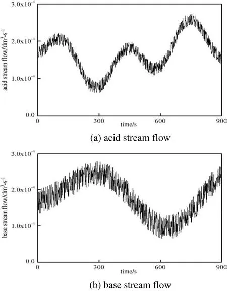
The p H neutralization happens with acid stream(H2SO4)and base stream(NaOH)mixed in the reactor of the laboratory(Department of Automation,China University of Petroleum Beijing),and this process is studied in this part.For this soft sensor system,the acid stream flow and base stream flow represent secondary variables(shown in Fig.3),and p H value represents the primary variable.

Fig.2.The identification procedure for soft sensor model.

This experiment is conducted for more than 30 min,and the fast sampling period is 3 s and the slow one is 6 s.150 groups of samples are used for model training.The p H value is sampled at slow sampling rate,and the acid and base stream flow are sampled at fast one.To illustrate the effectiveness of the proposed model in this study,SVM[4]and RBF-ARX-based[24]models are built for comparison.These two models are introduced as representative nonlinear model and the nonlinear dynamic one,respectively.At the same time,the trained SVM model serves as the secondary auxiliary model.In addition,the previous model with single time constant in our last studies[6,7]is also trained.

For SVM model,the most used Gaussian kernelis adopted here.The cross-validation strategy is used to determine the regularization parameter C,the precision threshold ε,and the kernel parameter γ.For RBF-ARX-based model,the structured nonlinear optimization method is utilized to determine the number of neurons and parameters.For the proposed model,the algorithms of Eqs.(13),(17)are used for obtaining the dynamic and static model parameters respectively with ρ(kq)=1/k.The final estimations for p H value based on the four models at fast sampling periods are shown in Fig.4.

Fig.3.Acid stream flow and base stream flow.

It is obvious from Fig.4 that the proposed model provides better estimations for the p H values with MSE(mean square error)=0.08.However,the estimation errors from the previous model,the RBFARX-based and SVM models are larger with MSE=0.17,0.5,0.8,respectively.Compared with the estimation results,the model in this paper shows more effectiveness for describing this soft sensor system.The SVM model could be actually regarded as a nonlinear model which only reveals the static relationship between input and output data.However,the p H neutralization process is always in dynamic state,and the sampled data contain dynamic information.Therefore,the SVM model may not estimate the p H value accurately.On the other hand,the ARX-RBF-based model incorporates the state dependent ARX model in nonlinear dynamics description and the RBF network in function approximation.The description of the static and dynamic characteristics of this process is integrated within the auto regression structure,which limits the estimation accuracy.Therefore,the proposed model structure does show more accuracy for this soft sensor system than the SVM and RBF-ARX-based models.Making comparison of the previous model and the improved one,we find that the improved one has smaller estimation error,which illustrates that the acid and base stream flows indeed affect the p H values in different speed.Therefore,taking multi-dynamic-characteristics into consideration does improve the accuracy of the model.

Fig.5 shows the action of auxiliary models(150 times in total),“1”represents that the secondary auxiliary model functions;otherwise,the primary one works.It can be seen that the secondary auxiliary model acts for twice,which indicates that there indeed exists the divergence of inters ample estimations from primary auxiliary model.Although the action number is few,the secondary auxiliary model is very critical to guarantee the identification process.On the other hand,it functions at the preliminary stage of the identification,and the inters ample estimations are obtained from the primary auxiliary model in most of the time.

Fig.4.p H values and model estimations.——:p H values;+:p H estimations.

Fig.5.Secondary auxiliary model function frequency.

7.Conclusions

In this paper,the separation of multi-dynamic and static characteristics based soft sensor model is proposed.The dynamic and static sub models build the dynamic and static relationships between secondary and primary variables respectively.The proposed model shows more effectiveness for describing soft sensor system,which has been confirmed in the laboratorial case.And the improvement makes the model more accurate and practical.Actually,we mainly focus on the concept and thought of the characteristics-separation-based model,rather than the specific expression.We hope this type of model has certain inspiration and help for soft sensor modeling.

We have made other contributions in this study.Given that the model structure,sub step identification mode is better for obtaining more accurate model parameters.Then,the SNR algorithm is studied and adopted.To guarantee the identification process,two auxiliary models are utilized to offer inter sample estimations in switching mechanism.And based on the auxiliary models,DAM-SNR algorithm is proposed and adopted for identifying soft sensor model together with the SNR algorithm.The double-auxiliary-model method is first put forward,and indeed gives great help for model identification.Although some development has been obtained,there are some shortages of the research in this paper.For example,The forgetting factor has great deal with the convergence speed and estimation error,and there must have the optimal choices for{ρ(kq)}.Therefore,some way should be found to determine the forgetting factor in real-time to adapt to working condition change.

[1]P.Kadlec,B.Gabrys,S.Strandt,Data-driven soft sensors in the process industry,Comput.Chem.Eng.33(2009)795–814.

[2]K.Fujiwara,M.Kano,S.Hasebe,Development of correlation-based pattern recognition algorithm and adaptive soft-sensor design,Control.Eng.Pract.20(2012)371–378.

[3]P.Facco,F.Doplicher,F.Bezzo,M.Barolo,Moving average PLS soft sensor for online product quality estimation in an industrial batch polymerization process,J.Process Control 19(2009)520–529.

[4]C.Shang,X.Gao,F.Yang,D.Huang,Novel Bayesian framework for dynamic soft sensor based on support vector machine with finite impulse response,IEEE Trans.Control Syst.Technol.24(4)(2014)1550–1557.

[5]J.Liu,Developing a soft sensor based on sparse partial least squares with variable selection,J.Process Control 24(2014)1046–1056.

[6]P.Cao,X.Luo,Modeling for soft sensor systems and parameters updating online,J.Process Control 24(6)(2014)975–990.

[7]P.Cao,X.Luo,Soft sensor model derived from Wiener model structure:modeling and identification,Chin.J.Chem.Eng.22(5)(2014)538–548.

[8]Y.Wu,X.Luo,A novel calibration approach of soft sensor based on multirate data fusion technology,J.Process Control 20(10)(2010)1252–1260.

[9]B.Lin,B.Recke,T.Schmidt,J.Knudsen,S.Jorgensen,Data-driven soft sensor design with multiple-rate sampled data:A comparative study,Ind.Eng.Chem.Res.48(2009)5379–5387.

[10]J.Wang,T.Chen,B.Huang,Multirate sampled-data systems:Computing fast-rate models,J.Process Control 14(2004)79–88.

[11]F.Ding,T.Chen,Combined parameter and output estimation of dual-rate systems using an auxiliary model,Automatica 40(10)(2004)1739–1748.

[12]F.Ding,T.Chen,Hierachical identification of lifted state-space models for general dual-rate systems,IEEE Trans.Circuits Syst.Regul.Pap.52(6)(2005)1179–1187.

[13]J.Ding,F.Ding,The residual based extended least squares identification method for dual-rate systems,Comput.Math.Appl.56(2008)1479–1487.

[14]H.Raghavan,B.Gopaluni,S.Shah,J.Pakpahan,R.Patwardhan,C.Robson,Gray-box identification of dynamic models for the bleaching operation in a pulp mill,J.Process Control 15(4)(2005)451–468.

[15]Y.Ma,D.Huang,Y.Jin,Discuss about dynamic soft-sensing modeling,J.Chem.Ind.Eng.56(8)(2005)1516–1519.

[16]C.Shang,X.Huang,A.Johan,D.Huang,Enhancing dynamic soft sensors based on DPLS:A temporal smoothness regularization approach,J.Process Control 28(2015)17–26.

[17]X.Gao,F.Yang,D.Huang,Y.Ding,An iterative two-level optimization method for the modeling of Wiener structure nonlinear dynamic soft sensors,Ind.Eng.Chem.Res.53(3)(2014)1172–1178.

[18]O.P.Ferreira,M.L.N.Goncalves,P.R.Oliveira,Local convergence analysis of inexact Gauss-Newton like methods under majorant condition,J.Comput.Appl.Math.236(9)(2012)2487–2498.

[19]A.D.Richard,Gauss-Newton and M-estimation for ARMA processes with in finite variance,Stoch.Process.Appl.63(1996)75–95.

[20]P.P.Khargonekar,K.Poolla,A.Tannenbaum,Robust control of linear time-invariant plants using periodic compensation,IEEE Trans.Autom.Control 30(1985)1088–1096.

[21]C.Shang,F.Yang,D.Huang,W.Lyu,Data-driven soft sensor development based on deep learning technique,J.Process Control 24(2014)223–233.

[22]H.Tian,S.David,S.Jang,Development of a novel soft sensor using a local model network with an adaptive subtractive clustering approach,Ind.Eng.Chem.Res.49(2010)4738–4747.

[23]O.Bruno,S.Walace,F.Alex,A.Luis,Data-driven soft sensor of down hole pressure for a gas-oil well,Control.Eng.Pract.22(2014)34–43.

[24]P.Hui,O.Tohru,T.Yukihiro,S.Hideo,N.Kazushi,H.Valerie,M.Masafumi,RBF-ARX model-based nonlinear system modeling and predictive control with application to a NOxdecomposition process,Control.Eng.Pract.12(2004)191–203.