Numerical study and acceleration of LBM-RANS simulation of turbulent flow☆

Shuli Shu,Ning Yang*

State Key Laboratory of Multiphase Complex Systems,Institute of Process Engineering,Chinese Academy of Sciences,Beijing 100190,China

1.Introduction

Fluid mixing is ubiquitous in chemical and process industries,and Computational Fluid Dynamics(CFD)is playing important roles in evaluating the mixing for various processes[1–3].Traditional Finite Volume(FV)-based CFD models prove to be feasible for the steady-state simulation of mixing processes or the transient simulation of physically fast mixing processes.In the latter case,the flow can reach equilibrium within a relatively short time and can be effectively simulated by traditional CFD with current computational resources.For instance,the mixing of two or more miscible fluids of similar densities or viscosities can be treated as a single-phase flow of multiple components,and the FV-based CFD simulation was always decoupled into two procedures:the flow field was first obtained through steady-state simulation,and then the scalar transport equations,e.g.,the concentration of components,were separately solved in a time-dependent manner with the calculated flow field[4–6].The computational resource needed is relatively small and some critical parameters such as mixing time can be predicted with certain accuracy[7,8].On the other hand,in case of two-phase flow such as the mixing of gas bubbles and liquids,the two- fluid models may have to be applied to differentiate the movement tendencies of the mixing fluids at the governing equations level[9,10],let alone Direct Numerical Simulation(DNS)[11]or Eulerian-Lagrangian simulation[12]of multiphase flow.In this case,the problems of higher computational cost and difficulties in numerical stability may become pronounced since the equations are strongly coupled,and the modeling accuracy is also sensitive to the turbulence models or inter phase interaction models.

However,for some mixing processes with highly transient characteristics or the so-called active mixing[13,14]in which the distribution of miscible solvent has non-negligible influences on flow field,even solving the equations of time-dependent single-phase turbulent flow of multiple components is time-consuming,let alone using the two- fluid models.A typical example is the mixing of crude oil in large–diameter storage tanks in which it takes hours or days to complete the mixing of two or multiple crude oils of different densities[15,16]and only the transient flow simulation is relevant.To effectively simulate the mixing of two crude oils of different densities in storage tanks with acceptable computational cost,the Boussinesq approximation is generally applied,keeping only the density difference in the gravitational term as a compromise between computational cost and accuracy[17,18].Even though,it is still unfeasible to simulate transient mixing processes in industrial scale by solving FV-based CFD.For example,it took about 30 CPU hours to update only one second of physical time when using FV-based CFD and Detached Eddy Simulation(DES)to solve the single-phase flow and scalar transport equations for the passive mixing process(the solvent distribution has less impacts on flow field)[13,14]in a cylindrical stirred tank(diameter T:0.15 m and height H=T,cells number:500000,time step:0.001 s)[19].For those active mixing processes,it may take about 432000 CPU hoursor more to simulate only oneday of physical time for crude oil mixing in a storage tank(more than 104m3),even using only 500000 cells in total.It is therefore not affordable or a challenging issue for traditional FV-based CFD methods to simulate transient mixing processes in such large-scale industrial applications.

The parallel computation of Lattice Boltzmann Method(LBM)simulation accelerated by Graphic Processing Units(GPU)might be a suitable alternative.LBM is distinguished by the explicitly time marching and highly localized computation properties,and proves to be more suitable for parallel computation and transient flow simulation[20,21],in particular when utilizing the modern high performance GPU cards.The computational speed of GPU-accelerated LBM is reported to be able to achieve nearly two-orders of magnitude faster than the LBM simulation using contemporary mainstream CPU[22].In addition,the flow in crude oil mixing process in industrial scale is always turbulent.Reynolds-Averaged Navier–Stokes(RANS)turbulence modeling is more practical and economical than DNS[17,18]or Large Eddy Simulation(LES)[23,24],and may also be the only feasible approach for large-scale industrial turbulent flow simulation.The standard k–ε model,the most popular RANS model,solves the transport equations of turbulent kinetic energy or turbulent dissipation rate[25].Compared to the FV-based CFD–RANS simulation,the GPU-accelerated LBM–RANS simulation is of practical interest for industrial applications.

Nevertheless,there are still several issues that need to be settled before exploiting the advantage of LBM–RANS simulation.First,to maintain the parallelism and computational efficiency of LBM,the RANS turbulence model may have to be explicitly solved.The LBM simulation using the Lattice Bhatnagar–Gross–Krook(LBGK)collision model has been coupled with the explicitly solved RANS model and validated in some benchmark problems of steady flow such as the turbulent pipe flows or separated flows[26,27]or the turbulent flow around the aircraft wing of NACA 4412 pro filed with surface grid re finement[28].However,the equations in RANS models,which consist of a set of non-linear source terms,are strongly coupled with each other and the momentum conservation equations.This nature of RANS models makes the explicit computation of RANS models difficult to converge[29].As a result,some artificial limitations were usually imposed for turbulent quantities to enhance the numerical stability.For example,the turbulent quantities were only allowed to be updated when the newly calculated turbulent viscosity was less than an upper threshold(e.g.,0.25 in lattice unit)[26],or the turbulent dissipation rateor turbulent kinetic energy was larger than alower threshold[28].The artificial numerical limitation may influence the accuracy of transient simulation,especially for the flow of longer evolution time in crude oil mixing.It is necessary to find a suitable combination of numerical treatments for the coupled model of LBM and explicitly solved RANS model,ensuring the numerical stability without resorting to the empirical artificial limitation.In this study,we first investigated the impacts of a series of factors such as the collision models in LBM,the discretization schemes of convection terms and the computational methods of production terms in standard k–ε model on numerical stability in a 2D case.These factors have not yet received a systematic study in the coupling of LBM and explicitly solved standard k–ε model.Rather than testing above-mentioned each single component which has been already reported in literature,we aim to find a suitable combination of these numerical schemes to ensure the numerical stability without any artificial limitations.A classical benchmark problem with complex flow separation,i.e.the turbulent flow over a backward-facing step was evaluated in the 2D simulations,and an optimized scheme combination was screened out for the 2D simulation cases.

Secondly,the optimized schemes for the 2D cases,however,still cannot guarantee the numerical stability in the 3D cases in our tests.Further refinement of the grids might improve the stability but at expense of much more computational resources.Hence it is still not suitable for the simulation of industrial-scale processes.To keep the numerical stability,the implicit method for RANS should be better,which may however greatly slowdown the computational speed and compromise the advantage of explicit computation and parallelism of LBM.The key question is how to harmonize the explicitly solved LBM and implicitly solved RANS to accelerate the computation.We then proposed a new accelerating method to synchronize the LBM and RANS computations,or in other words,making the RANS simulation compatible with the LBM computation.This method shows the potential to be applied for accelerating the computation of longtime active mixing processes in an industrial-scale mixing tank.

2.Mathematical Models

2.1.The Lattice Boltzmann Method

The governing equation of the Multiple Relaxation Time(MRT)–LBM[30,31]is

where f is the velocity distribution function vector,eiis the discrete velocity vector,M is the transformation matrix,and S is the diagonal collision matrix with adjustable parameters.m,the velocity distribution function vector in moment space,is computed by m=M f.meqis the equilibrium moment,I is the identity matrix,and F is the force term in moment space[32].The D2Q9 model is chosen for 2D simulation.The details of meq,M and F for 2D simulation are shown in Appendix.The parameters in S are set as S0=S3=S5=0,S1=1.19,S2=1.4,S4=S6=1.2 and Sv=S7=S8=1/τ0.For 3D simulation,the D3Q19 model is chosen.The parameters in S are set as S1=1.19,S2=S10=S12=1.4,S0=S3=S5=S7=0,S4=S6=S8=1.2,Sv=S11=S13=S14=S15=1/τ0and S16=S17=S18=1.2.The details of meq,M and F for 3D simulation are also shown in Appendix A.τ0is related to the kinematic viscosity of fluid v0=(τ0− 0.5)/3.In LBGK model,the parameters of S are all the same and equal to 1/τ0.For the LBM–RANS coupled modeling,the turbulent viscosity is integrated into the relaxation time by,

2.2.Turbulence modeling

2.2.1.The standard k–ε models

The transport equations for k and ε are generally formulated as

and

where σk0,σk,σε0,and σεare the model parameters.The turbulence viscosity

where Cμis the model parameter.The source terms Skand Sεfor the standard k–ε model are given as

Gk=and represent the generation of turbulence kinetic energy(production term)is the magnitude of strain rate tensor and=(2SijSij)1/2,andThe strain rate tensor can be calculated either from the central differencing or other Finite Difference Method(FDMs)for the macro-scale velocity variables,or from the local non-equilibrium part of velocity distribution function(NEQM)[33],

and.The model parameters in the standard k–ε model σk0= σk= σε0=1.0,σε=1.3,c1=1.44,c2=1.92 and Cμ=0.09.

2.2.2.Wall function

Since the flow is not turbulent all the way down to the wall,the wall functions were used to describe the law-of-the-wall velocity pro file through the empirical correlations to model the viscosity-dominated region.If the wall-adjacent nodes meet the law-of-the-wall rule,the shear stress at wall τwis equal to that at wall-adjacent nodes.The law-of-the wall for mean velocity for standard wall function is

where

and the von Karman constant κ=0.4178,B=5.0,UPis the velocity of fluid at the first wall-adjacent node P,kPis the turbulence kinetic energy of the first wall-adjacent node,yPis the distance between wall and the first wall-adjacent node.These relationships apply only when y+is between 11.5 and 300.Thereafter the shear stressat the wallτwcan beobtained.Then the production of kinetic energy Gk,under the hypothesis of local equilibrium at the wall-adjacent nodes,can be calculated from,

and the turbulent dissipation rate,

2.3.Numerical discretization of standard k–ε model

In this work,the standard k–ε model was solved by Finite Volume Method(FVM),and Eqs.(3),(4)can be rewritten as[26,27],

where ϕ represents the turbulent properties k or ε,Dϕis the effective viscosity and Sϕis the source term.Eq.(14)can be discretized as,

where aP=∑anb+-Sp,anbis the coefficient for neighboring nodes and depends on the discretized schemes.=ΔV/Δt anddenotes the turbulent variable in the last time step.For the k equation,Sc=Gkand SP=−,where k*is the turbulent kinetic energy of the last time step.For the ε equation,Sc=c1εGk/k and SP= −c2ε*/k,and ε*is the turbulent dissipation rate of the last time step.

3.Evaluation of Different Numerical Treatments

In this section,we investigated the influence of several key factors on the numerical stability of the coupled model of LBM and explicitly solved standard k–ε model,e.g.,the collision models in LBM,the discretization schemes of convection terms and the computational methods of production terms in the standard k–ε model.The impacts of the artificial limits were also investigated.For the collision models in LBM,we compared the simulation using the LBGK model with that of the MRT model.For the discretization schemes of the convection term in the standard k–ε model,we used the second order Total Variation Diminishing(TVD)scheme with SUPERBEE limiter[34]or the Weighted Essentially Non-Oscillatory(WENO)scheme[35].For the computation of production terms in the standard k–ε model,e.g.Gkin Eqs.(6),(7),we compared the FDM for macro-scale velocity variables and the NEQM from the LBM simulation(Eq.(8)).Rather than testing each single numerical method mentioned above which has been already investigated in literature,we aim to find a suitable combination of these numerical schemes,which can ensure the numerical stability of the coupled model without any artificial limitations.A classical turbulent flow benchmark problem with flow separation or turbulent backward-facing step flow has been used in the numerical tests.

The simulation was implemented on the supercomputer cluster“Mole-8.5”installed with a hybrid architecture of multiple Graphical Processing Unit(NVidia Tesla C2050 GPU)cards and CPU cores(Intel Xeon E5430 CPU,RAM 16G)in the Institute of Process Engineering of Chinese Academy of Sciences.It took about 67.5 s to update 10000 time step for the grid of 300×2000 with 4 GPU cards.It should be pointed out that the suitable load has to be chosen for GPU to achieve the maximum performance.We implemented the parallel computation of the coupled model of LBM and the explicitly solved standard k–ε model with the following steps:

(1)Decompose the whole domain into several sub-domains for parallel computation and initialize the variables on CPUs and GPUs;

(2)Update the velocity distribution function by calculating the collision process,i.e.,the right hand side of Eq.(1),f∗(x,t)=f(x,t)−M−1S(m−meq)+(I−S/2)F,and then the propagation process is implemented through f(x+eiΔt,t+Δt)=f∗(x,t).Here the turbulent viscosity is incorporated into the collision matrix S.This step is implemented on GPUs.

(3)Exchange and update the velocity distribution functions of sub

domain boundary on GPUs:the velocity distribution functions for data transfer stored on GPUs is first copied to the local CPUs,and then transferred to corresponding CPUs for the adjacent sub-domains using Message Passing Interface(MPI),and finally the velocity distribution functions on those CPUs is copied to their local GPUs allocated to the adjacent sub-domains to update the velocity distribution functions at the sub-domain boundary.

(4)Impose the boundary conditions and compute the macro variables,density fluctuations or velocity on GPUs;

(5)Update the turbulent kinetic energy k or turbulent dissipation rate ε through Eq.(15)and turbulent viscosity through Eq.(5)on GPUs;

(6)Exchange and update k and ε on sub-domain boundary as step 3;

(7)Return to step 2 and repeat steps 2–6 until the finalization of calculation.

3.1.Geometry and numerical setups

The geometry of backward-facing step flow is illustrated in Fig.1.The expansion rate(ER)is defined by ER=(Hin+H)/Hin=1.5 where Hinis the inlet height and H is the step height.L1=H and L2=20H.The flow condition is the same with the experiments[36]and the Reynolds number ReHbased on the step height H and free stream velocity(U0)is 44000.

The velocity inlet condition and the fully-developed outlet boundary condition were used.The stream-wise velocity distribution at inlet was set to follow the−1/7 law[37],

where U0is the fully-developed freest ream velocity and set as0.1 in lattice unit in all simulations,y is the distance between wall and nodes,δ is the boundary layer thickness and equal to Hin/3.3.The rest of boundaries are treated as no-slip walls.

The turbulent kinetic energy at the inlet kin=1.5I2U02and the turbulent intensityThe turbulent dissipation rate at inletand the length scale l=min(κy,0.085Hin/2)where the von Karman constant κ=0.4178 and y is the distance between the wall and first wall-adjacent nodes.Neumann boundary condition(the gradient of k and ε is zero)was imposed for k and ε at the outlet.It should be pointed out that the no-slip wall boundary condition is realized by the half-way bounce-back,and the wall is located at the half lattice height away from the first wall-adjacent nodes.Hence the calculation was not implemented all the way down to the wall,and the standard wall function was applied.

3.2.Effects of collision models

In the comparison of the collision models(LBGK and MRT),NEQM(Eq.(8))and TVD were used.The upper threshold limiter for turbulent viscosity was set as 0.25(in lattice unit),which follows the work of Teixeira[26].Fig.2 shows the convergence history of simulations with different collision models.The L2 error is defined by

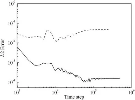
Fig.2.Convergence history when using different collision models.

Both the simulation cases converged.The L2 errors of the MRT–NEQM–TVD case are about two-orders smaller than that of the LBGK–NEQM–TVD case.Fig.3 illustrates the streamlines predicted in the two cases when the flow reaches the steady state.The MRT case is more stable and can qualitatively capture the primary and the secondary vortexes.By contrast,there are strong numerical oscillations in the LBGK simulation and even the primary vortex is not qualitatively captured.Then we compared the predicted vertical velocity at x/H=4,as illustrated in Fig.4.Fig.5 depicts the prediction of stream-wise velocity distribution at the bottom wall along the upstream of the step.Apparently,serious numerical oscillations appear in the LBGK simulation whereas the MRT case can eliminate this problem.

We further investigated the numerical stability of LBGK or MRT collision models coupled with other combination of numerical treatments,e.g.,the discretize schemes for convection terms(TVDor WENO)or production terms(2nd or 4th order FDM or NEQM).The artificial upper threshold limiter for turbulent viscosity(0.25 in lattice unit)was imposed in the simulations.As illustrated in Fig.6,for the LBGK collision model,the simulation only converges when TVD and NEQM methods are used for the standard k–ε model.Comparison of different numerical schemes is also listed in the table in Fig.6.By contrast,when using the MRT collision model,the simulation always converges(Fig.7).The simulation is more stable for the cases of MRT collision models.It should be noticed that these conclusions are made when the threshold limiters are imposed for turbulent viscosity.

3.3.Effects of threshold limiters

The artificial limitations on turbulent viscosity were employed to enhance the numerical stability,and the maximum turbulent viscosity at steady state was 0.07 in lattice units in the last section.These threshold limiters in literature are sometimes artificial or empirical and may affect the numerical accuracy,especially for the transient or time-dependent flow simulation.Then we investigated the effects of the upper threshold limiter(Mu)of turbulent viscosity.The upper limiter was used as a threshold in calculation to allow the update of the turbulent quantities.Three thresholds of turbulent viscosity(0.01,0.07 or 0.1 in lattice unit)were tested in the simulation in the MRT cases.As illustrated in Fig.8,the stream-wise velocity for Mu=0.07 are similar to that of Mu=0.1 at x/H=12(behind the step)and y/H=0.25.But there are large oscillations for Mu=0.01.It is clear that the threshold limiter does impact the transient flow simulation.

Fig.1.Geometry of backward-facing step flow.

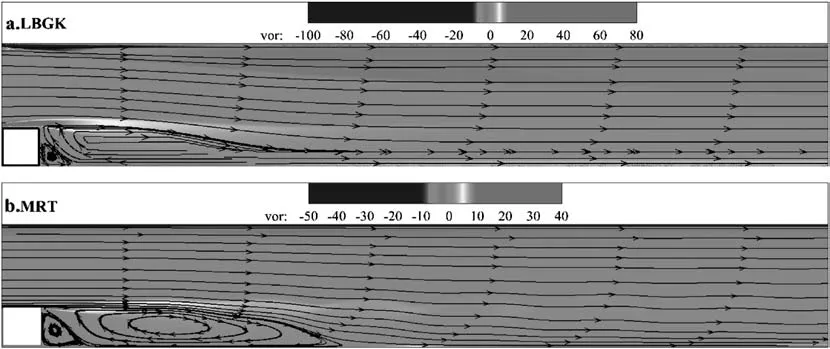
(a.LBGK–TVD–NEQM;b.MRT–TVD–NEQM).

Fig.4.Normalized vertical velocity(x/H=4).

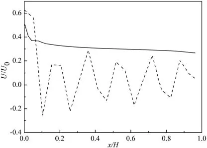
Fig.5.Normalized stream-wise velocity distributions(0＜x/H＜1 and y/H=1).

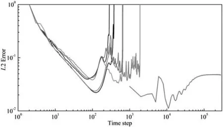
Fig.6.Convergence history when using LBGK collision model(threshold limiter for turbulence viscosity:0.25).

3.4.Effects of the computational methods for production term

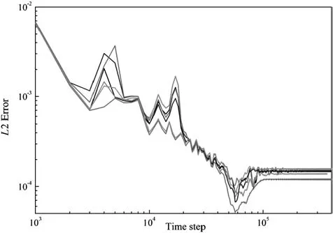
Fig.7.Convergence history when using MRT collision model(threshold limiter for turbulence viscosity:0.25).

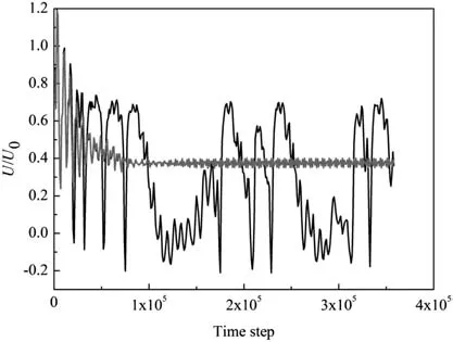
Fig.8.Stream-wise velocity when using different thresholds(Mu)for turbulent viscosity(x/H=12,y/H=0.25).

As mentioned in Section 3.2,only the cases jointly using the NEQM and TVD methods can converge when imposing the threshold limiter in the LBGK case,and there is no such limitation in the simulation of the MRT case.The latter suggests also that NEQM is not necessary to enhance the convergence of the MRT case.In this section,we then removed the artificial threshold limiters.As illustrated in Fig.9,the LBGK–NEQM–TVD case diverged.The cases using the MRT collision model and the TVD scheme for convection terms was always stable regardless of the discretization schemes for the production terms.The cases using MRT and WENO schemes for convection terms was only stable when NEQM was chosen to calculate the production terms.It can be found that both TVD and NEQM are necessary to ensure the convergence of the MRT cases without the threshold limiters for turbulent viscosity.

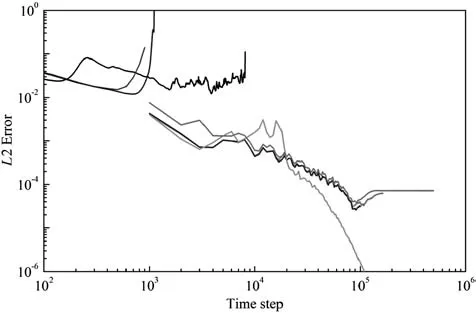
Fig.9.Convergence history when using different numerical treatments(without threshold for turbulence viscosity).

3.5.Boundary layer

The grid configuration,especially the arrangement of wall-adjacent nodes,is important for simulation accuracy.It was reported that the grid-independent solution for the flow with separation,such as backward-facing step flow,cannot be obtained for most of the turbulence modeling approaches using wall functions or even the k–ω model[38].To investigate the effect of boundary layer modeling,the MRT–TVD–NEQM method which shows the best numerical stability without imposing the threshold limiters for turbulence viscosity,was used in this section.The first wall-adjacent nodes should be located in the logarithmic region,which means that y+should fall in the range of 11.5–300.y+can be estimated from the correlation,y+≈[39].Hence the distance between the first wall-adjacent node and wall Δy meets the condition:Δy is 0.5 in lattice unit when using the half-way bounce-back boundary condition and uniform grid in this simulation.The height of inlet in lattice unit meets the following constraint,which means that the maximum grid number for Hinis around 200 in lattice unit.The effect of mesh size on the predicted reattachment length by the standard k–ε model with wall functions is shown in Fig.10.The prediction deviates from the experimental data within±10%when y+of the wall adjacent nodes in front of the step is about 9–15.Further grid refinement cannot improve the simulation results when y+is smaller than 9.Hence 30–50 lattice grids along the step height is suitable for the reattachment length predictions,and the simulation in the following sections then placed 40 grids along the step height direction.

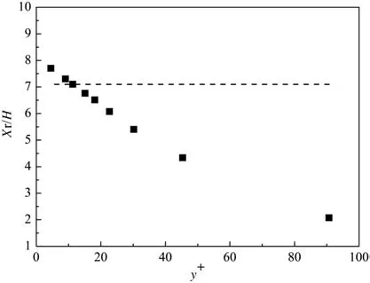
Fig.10.Normalized reattachment length(Xr/H).

Overall,in the above LBM simulations coupled with the explicitly solved RANS model,the MRT collision model together with the TVD scheme for convection terms and NEQM scheme for production terms(MRT–TVD–NEQM)with 40 grids along the step height is more stable without the need to impose the threshold limiters for turbulent quantities,and therefore could be recommended for the explicitly solved LBM–RANS.Fig.11 shows the streamline of the steady flow predicted in this work and two other simulations in literatures using Re-Normalization Group(RNG)k–ε model[26]or k–ω model[27].The reattachment length for primary vortex predicted in this work was 7.09.The reattachment length predicted in the literature was 7.20 for RNG k–ε model[26],7.00 for k–ω model[27].The reattachment length predicted by this work seems to be in better agreement with the experiments(7.10)[36]than the other two.The secondary vortex at the corner behind the step can be captured,which cannot be observed in the other two simulations[26,27].This can also be seen from Fig.3 that the secondary vortex cannot be clearly captured by LBGK–TVD–NEQM though the calculation could converge.We found that the evolution of the secondary vortex was slower than that of the primary vortex,and it took longer time for the secondary vortex to reach steady state than the primary vortex,and the evolutions of secondary vortex did not change the reattachment length of the primary vortex.

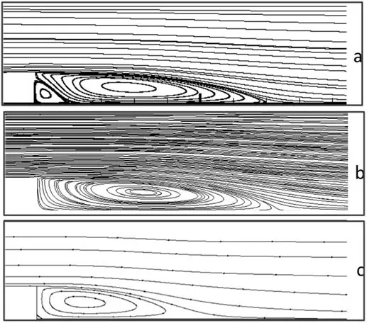
(a)this work:2D-MRT–TVD–NEQM,standard k–ε;(b)2D-LBGK,RNG k–ε model,PGE-LW wall model[26];(c)2D-LBGK,k–ω or Spalart-Allmaras turbulent model[27].

The stream-wise velocity distribution behind the step is presented in Fig.12.The prediction of the hybrid model coupling LBM and standard k–ε model with the recommended scheme is in good agreement with the experiments[36].

Then we employed the MRT–TVD–NEQM scheme for the flow at higher Reynolds number(up to 10 million).40 uniform grids were placed along the step height.No threshold limiters were imposed for the turbulent quantities.The streamline and vorticity contour predicted by the MRT–NEQM–TVD scheme at Re=107is depicted in Fig.13.The 2D simulation can still converge for such high Reynolds number flow.

It should be pointed out that for the 3D simulation of high Reynolds numbers backward facing step flow using LBM and the explicitly solved standard k–ε model,even the above scheme optimized for 2D case may not guarantee the computational convergence of 3D cases.It is generally acknowledged that 2D simulation is more stable than 3D simulation.3D cases are more complicated and always require stricter CFL criteria to ensure the convergence of the explicit simulation.Mathematically,it is still not well understood about the dominating factor that impacts the numerical stability in the coupling of LBM and standard k–ε model.A number of factors may affect the numerical stability of this coupling such as grid size,time steps,discretization schemes,dimension of computational domain,or symmetry of lattice model.For the latter case,the artificial limitation for turbulent quantities or using the lattice models of more discrete velocities may still be required for coarse grid calculation.Theoretically,the 3D explicit simulation may converge with finer grid and smaller time steps,but at the expense of huge computational costs,which is not feasible for industrial application and therefore not the purpose of this paper.To seek a practical approach for 3D cases,we returned back to the implicit method in solving the standard k–ε model.The implicit method needs more iterations and discount the advantage of the explicit computation of LBM.Section 4,therefore,tackles the acceleration of the coupling of LBM and the implicitly solved standard k–ε model for 3D cases.

4.A New Acceleration Method for Implicit 3D Simulation

When the RANS turbulence model is implicitly solved,the LBM–RANS simulation is more stable and does not require the artificial numerical limitation.However,there are still several open questions.The implicit method in the RANS simulation always needs many more iterations to ensure the computational convergence and the computational speed is relatively much slower.The LBM simulation,on the other hand,is an explicitly time-marching approach with much faster computational speed.Moreover,the grid size and the time step in LBM simulation are constrained to ensure the numerical stability of LBM.However,there are no such restrictions on the grid size or time step in implicitly solved RANS turbulence model.In the coupling of LBM and RANS,these models are generally solved using the same spatial or temporal steps.The above constraint in the implicitly solved procedure of RANS model may greatly slowdown the LBM–RANS computation and counteract the advantage of parallelism of LBM.

Fig.12.Stream-wise velocity distribution.

Fig.13.Streamline and vorticity contour predicted by MRT–NEQM–TVD(without threshold)at Re=107.

The key issue is how to find a compatible approach for both the models and meanwhile accelerate the computation.In this work,we propose a new acceleration method to synchronize the LBM and RANS computations,or in other words,making the RANS simulation compatible with the LBM computation.In this method,the RANS model is solved at relatively larger time steps,where as the LBM simulation is implemented on smaller time steps to ensure the numerical stability due to the explicitly time-marching properties.For the two-way coupling of the LBM and implicitly solved RANS model,the turbulent viscosity from RANS model is needed to modify the relaxation time in LBM,and the fluid velocity is needed in RANS.In our calculation,the turbulent viscosities were only stored or updated at larger time steps in RANS and the fluid velocities were updated at smaller time steps in LBM.This new method is a compromise between computational efficiency and accuracy,and suitable for the simulation problems with a set of coupled equations in which some equations are simple to solve and can be computed fast and the remaining equations are complex and time consuming.The computational speed is dominated by the time-consuming equations.It should be noticed that we still use the same grid configuration for both the LBM and RANS simulation.Actually extension of the above method in terms of spatial scales is straightforward and the spatial interpolation method is required in this case.

To clarify and test the new method,we simulate the transient active mixing process of two fluids with different densities in a cubic domain(～10 m in each direction)using the LBM–RANS(implicitly-solved standard k–ε turbulence model)model.The LBM–RANS simulations were compared with the FV-based CFD simulation using commercial software ANSYS Fluent®to test its accuracy and computational efficiency.This simulation was carried out for the mixing process of two different types of miscible fluids in a mixing tank.The Boussinesq approximation was applied and the density difference of the two fluids was neglected in governing equations,which means the density kept constant in calculations.Atwood number,A=(ρ1− ρ2)/(ρ1+ ρ2),is always used to represent the density difference of two fluids in Boussinesq approximation method in literature[40].Although A→0 can give better prediction,this method was also extend to simulate the flow with high Atwood number,e.g.,0.16[41]and 0.5[40].The influence of density variations was taken into consideration by the buoyance force,Fb,

where α is the volume fraction of the other fluid,Δρ is the density difference of the two fluids,and g is gravity acceleration.

The scalar transport equation of α is

where Γ is the eddy diffusivity,and the ratio between the turbulent viscosity and eddy diffusivity is the Schmidt number(Sc).The viscosity of the mixture was updated in term of the local volume fractions of different fluids.The transport equation was coupled with the governing equations of fluid flow(Eq.(1))and the standard k–ε turbulence models.Both the scalar transport equations and the standard k–ε models were implicitly solved by FVM.

We differentiated two time scales to solve the integrated equations,and the spatial resolution for the equations was kept the same.For the LBM equation,the time step d t0was smaller(e.g.,0.002 s).For the scalar transport equation and implicitly solved standard k–ε model equations,the time step d t1(e.g.,0.1 s)was set to be much larger than dt0.An integral ratio of d t1to d t0(n)was always chosen for convenience.Only when the scalar transport equations and the LBM equations were solved by n time steps(n d t0),the standard k–ε model equations started to be solved for one time step d t1to update the turbulent viscosity.The new method essentially realizes the synchronization of computational or evolutional speed of the different equations through the difference in time steps.In this way,the RANS,LBM and scalar transport equations can be solved in a synchronous manner to maintain the highly parallel computational efficiency and meanwhile the numerical stability.It is also physically reasonable since RANS is a time-averaged model and can be solved at a relatively larger temporal scale.

4.1.Computational acceleration estimation

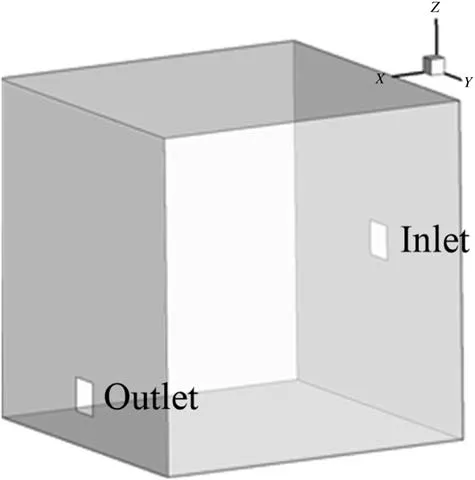
Fig.14.Geometry of the cubic flow domain.

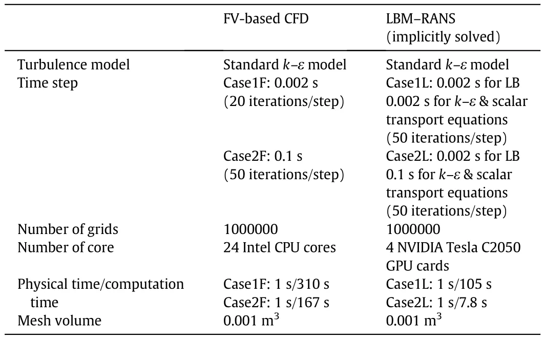
Table 1 Numerical setup and computational speed for mixing process

In this section,computational time for mixing process in a cubic tank was compared with Ansys Fluent®simulation and the original coupled model of LBM and the implicitly solved RANS to demonstrate the computational efficiency of the new acceleration method proposed in this study.The cubic flow domain(10 m×10 m×10 m)is depicted in Fig.14,and the spatial scale is similar to the mixing tank of crude oils.The size of inlet and outlet were 1 m×1 m.The distance to the bottom plane was5 m for the inlet and 1.5 m for the outlet.Initially,the flow domain was filled with heavy fluid(density:900 kg·m−3,kinematic viscosity:1.5 × 10−4m·s−2).A light fluid(density:640 kg·m−3,kinematic viscosity:1.5×10−4m·s−2)was pumped into the cubic domain and two fluids were mixed.The two fluids were miscible and the corresponding Atwood number was 0.17.A classical Sc number(1000)for liquid–liquid mixing process was used,and the inlet velocity was 5 m·s−1.

We compared the computational speed of the new acceleration method with the previous method for solving the LBM–RANS model.The computational accuracy was validated by comparing the LBM–RANS simulation with the FV-based CFD simulation using commercial package ANSYS Fluent®.Four cases(case1L,case2L,case2F and case2F)were set up to test the computational speed and accuracy.Case1L adopted the previous coupling method for the LBM–RANS simulation and all the equations were solved by using the same time step and grid size.Case2L implemented the new acceleration method.Case1F and Case2F are the FV-based CFD simulations using ANSYS Fluent®in which the time step or grid size were kept the same for both the fluid solver and the turbulence model equations.The time step in Case1F was much smaller than Case2F.The grid size in the LBM–RANS simulation was uniform(0.1 m),the same with the FV-based CFD simulations.The detail of numerical setup is shown in Table 1.

In Case2F and Case2L,the time step was enlarged to 0.1 s and the iteration number within each time step was also enlarged to keep the numerical stability.As illustrated in Table 1,although the time step in Case2F was 50 times larger than Case1F,the computational speed of Case2F was only 1.86 times faster than that of Case1F,and the computation cannot be linearly accelerated by simply increasing the time step.On the other hand,the computational speed of Case2L was nearly 13.5-fold faster than Case1L,which means that the new acceleration method can significantly promote the computational speed and efficiency.The accuracy of the new acceleration method(Case2L)was compared with the FV-based CFD simulation(Case1F),as illustrated in Fig.15.We can find that the new acceleration method is in reasonably good agreement with the FV-based CFD simulation.The light crude oil tends to flow up to the top of flow domain due to the buoyancy effects.One can further choose the high order temporal or spatial discretized schemes to optimize or improve the simulation accuracy.Theoretically,the new method is suitable not only for the coupling of LBM and the standard k–ε model,but also for the coupling of LBM with other RANS models with non-linear terms.It should be noted that for the crude oil mixing,it may take several hours or days to achieve a complete mixing degree.In the FV-based CFD simulations,even for such a smaller-scale mixing tank(10 m×10 m×10 m),it still takes about 310 days to update the simulation of physical time of one day.By utilizing the new acceleration method for LBM–RANS,we only need about 1 week.

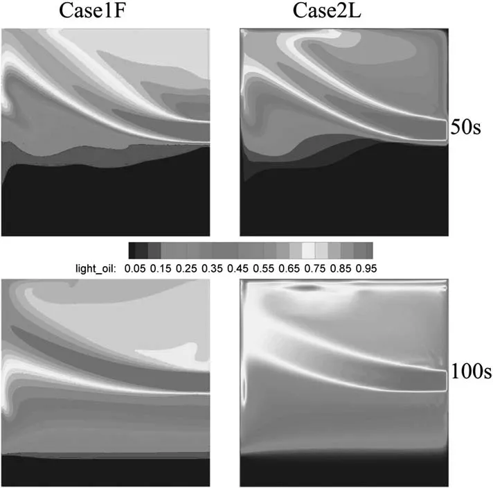
Fig.15.Temporal evolution of light oil concentration.Left:Case1F(bottom);Right:Case2L,LBM–RANS with the new acceleration method.

5.Conclusions

With natural parallelism and explicit time-marching properties,the LBM–RANS models may hitherto be more practical and economical for LBM methods to be applied in industrial-scale turbulent flows,despite the active researches on DNS or LES in academia.To keep the efficiency of parallel computation of LBM,the RANS model should also be explicitly solved,which greatly affects the numerical stability;whereas to keep the numerical stability,the implicit method should be better for RANS,which compromises the advantage of explicit computation and parallelism of LBM.To deal with the real world applications,the key is howto enhance the numerical stability for the coupled model of LBM and the explicitly solved RANS,or to harmonize LBM and the implicitly solved RANS to synchronize the LBM and RANS computation.For the explicitly solved standard k–ε model,we found that those artificial limitations imposed on turbulent quantities to improve numerical stability may influence the accuracy of transient simulations.The combination of MRT and TVD or MRT and NEQM can ensure computational convergence without the need to impose artificial limitations in the 2D simulation of backward-facing step flow.The MRT–TVD–NEQM scheme was stable even at Re=10000000 in 2D simulation.But the scheme may still not guarantee the convergence of 3D simulation in feasible computational resource requirement.Then we proposed a new acceleration method to synchronize the LBM and RANS computation,solving the RANS model at relatively larger time steps and the LBM equation at smaller time steps,and implemented this method for the LBM coupled with implicitly solved standard k–ε model.This new method was successfully implemented by GPU-accelerated computation for an industrial-scale tank for crude oil mixing.The computational speed was about 13.5-fold faster than the GPU computation of LBM–RANS without using this method,and 40-fold faster than the parallel computation using the FV-based CFD simulation of commercial CFD software and multiple CPUs.

Nomenclature

aPCoefficient of node P in discretization

anbCoefficient of neighborhood nodes in discretization

B Model parameter(=5.0)

CμModel parameter in RANS model(=0.09)

c1Model parameter in RANS model(=1.44)

c2Model parameter in RANS model(=1.92)

D2Q9 Lattice model in 2D

D3Q19 Lattice model in 3D

Dϕthe effective viscosity

ER Expansion rate(=1.5)

eiDiscrete velocity vector,m·s−1

F Force term in moment space

f Velocity distribution function vector

GkGeneration of turbulent kinetic energy

g Gravity acceleration,m·s−2

HinInlet height,m

I Turbulent intensity

k Turbulent kinetic energy,m2·s−2

kPTurbulent kinetic energy at node P,m2·s−2

L2 L2 error norms

l Length of scale

M Transformation matrix

m Velocity distribution function vector in momentum space

meqEquilibrium moment

ReReynolds number

ReHin Reynolds number based on height of inlet

S Diagonal collision matrix with adjustable parameter

S Magnitude of strain rate tensor,s−1

ScSchmidt number

SijStrain rate tensor's components,s−1

SkSource term in k equation

SεSource term in ε equation

U0Fully-developed free stream velocity,m·s−1

UPThe velocity of fluid at the first wall-adjacent node P,m·s−1

uiFluid velocity in i direction,m·s−1

u+Non-dimensional velocity

v0Non-dimensional kinematic viscosity of fluid

vtTurbulent kinematic viscosity,m2·s−1

XrReattached length,m

y Distance between wall and nodes,m

yPDistance between node P and wall,m

y+Dimensionless wall distance

α The volume fraction of fluid

Γ Eddy diffusivity,m2·s−1

δ The boundary layer thickness,m

ε Turbulent dissipation rate,m2·s−3

εinTurbulent dissipation rate at inlet,m2·s−3

εPTurbulent dissipation rate at node P,m2·s−3

κ Von Karman constant(=0.4178)

Δρ Density difference,kg.·m−3

σkModel parameter in RANS model(=1.0)

σk0Model parameter in RANS model(=1.0)

σεModel parameter in RANS model(=1.3)

σε0Model parameter in RANS model(=1.0)

τ0Non-dimensional relaxation time

τwShear stress at the wall,kg·m−1·s−2

ω The specific rate of dissipation,s−1

Appendix

For D2Q9 model,the transformation matrix,M,is written as,

The corresponding discrete velocity eiis written as,

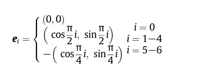
The equilibrium moment,meq,is meq=(δρ,−2δρ+3u2,δρ−3u2,ux,−ux,uy,−uy,−,uxuy).

The force,F,in moment space is,

For D3Q19 model,the transformation matrix,M,is written as,

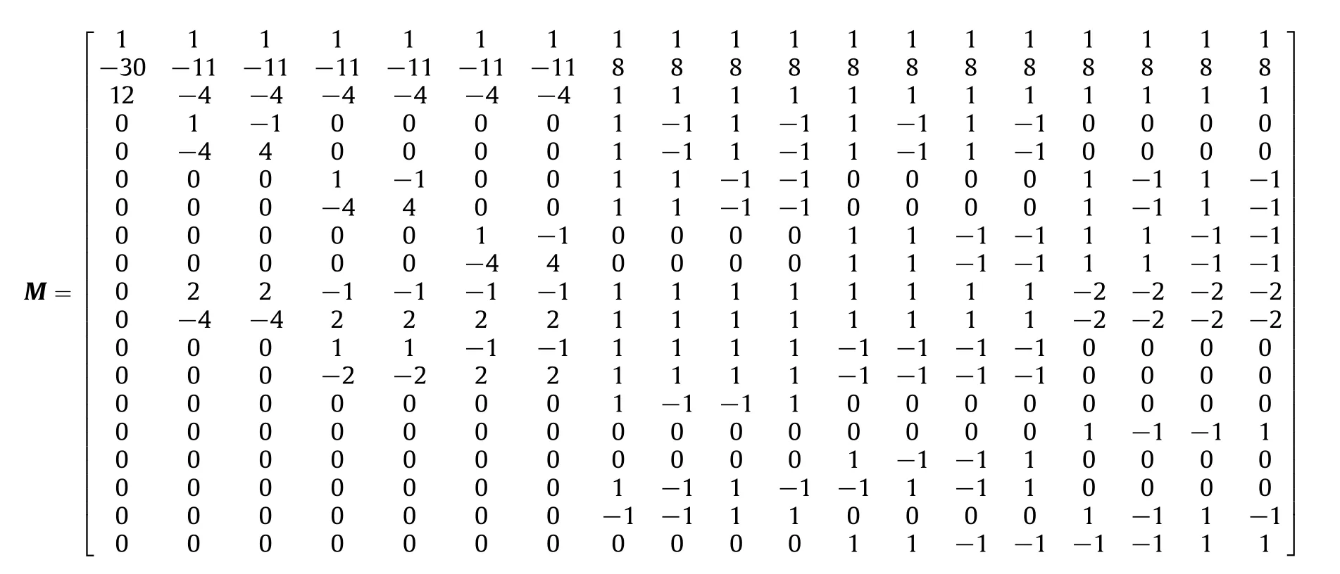
The corresponding discrete velocity e is written as,

The equilibrium moment,meq,is written as,

The force,F,in moment space is,

[1]L.Fradette,P.A.Tanguy,F.Bertrand,F.Thibault,J.-B.Ritz,E.Giraud,CFD phenomenological model of solid–liquid mixing in stirred vessels,Comput.Chem.Eng.31(2007)334–345.

[2]S.Jayanti,Hydrodynamics of jet mixing in vessels,Chem.Eng.Sci.56(2001)193–210.

[3]A.W.Patwardhan,CFD modeling of jet mixed tanks,Chem.Eng.Sci.57(2002)1307–1318.

[4]M.Rahimi,A.Parvareh,Experimental and CFD investigation on mixing by a jet in a semi-industrial stirred tank,Chem.Eng.J.115(2005)85–92.

[5]D.Cheng,X.Feng,J.Cheng,C.Yang,Numerical simulation of macro-mixing in liquid–liquid stirred tanks,Chem.Eng.Sci.101(2013)272–282.

[6]J.M.Bujalski,Z.Jaworski,W.Bujalski,A.W.Nienow,Fluid mixing VII The influence of the addition position of a tracer on CFD simulated mixing times in a vessel agitated by a Rushton turbine,Chem.Eng.Res.Des.80(2002)824–831.

[7]J.Min,Z.Gao,Large eddy simulations of mixing time in a stirred tank,Chin.J.Chem.Eng.14(2006)1–7.

[8]Q.Zhang,Y.Yong,Z.-S.Mao,C.Yang,C.Zhao,Experimental determination and numerical simulation of mixing time in a gas–liquid stirred tank,Chem.Eng.Sci.64(2009)2926–2933.

[9]Q.Xiao,N.Yang,J.H.Li,Stability-constrained multi- fluid CFD models for gas–liquid flow in bubble columns,Chem.Eng.Sci.100(2013)279–292.

[10]N.Yang,Z.Wu,J.Chen,Y.Wang,J.Li,Multi-scale analysis of gas–liquid interaction and CFD simulation of gas–liquid flowin bubble columns,Chem.Eng.Sci.66(2011)3212–3222.

[11]S.L.Shu,N.Yang,Direct Numerical Simulation of Bubble Dynamics Using Phase-Field Model and Lattice Boltzmann Method,Ind.Eng.Chem.Res.52(33)(2013)11391–11403.

[12]L.M.Wang,B.Zhang,X.W.Wang,W.Ge,J.H.Li,Lattice Boltzmann based discrete simulation for gas-solid fluidization,Chem.Eng.Sci.101(2013)228–239.

[13]S.P.Sullivan,B.S.Akpa,S.M.Matthews,A.C.Fisher,L.F.Gladden,M.L.Johns,Simulation of miscible diffusive mixing in microchannels,Sens.Actuators B Chem.123(2007)1142–1152.

[14]G.Ivey,K.Winters,J.Koseff,Density stratification,turbulence,but howmuch mixing?Annu.Rev.Fluid Mech.40(2008)169–184.

[15]A.A.Dakhel,M.Rahimi,CFD simulation of homogenization in large-scale crude oil storage tanks,J.Pet.Sci.Eng.43(2004)151–161.

[16]M.Rahimi,A.Parvareh,CFD study on mixing by coupled jet-impeller mixers in a large crude oil storage tank,Comput.Chem.Eng.31(2007)737–744.

[17]J.J.Derksen,Blending of miscible liquids with different densities starting from a stratified state,Comput.Fluids 50(2011)35–45.

[18]J.J.Derksen,Direct simulations of mixing of liquids with density and viscosity differences,Ind.Eng.Chem.Res.51(2012)6948–6957.

[19]F.Yang,S.Zhou,G.Wang,Detached eddy simulation of the liquid mixing in stirred tanks,Comput.Fluids 64(2012)74–82.

[20]S.Chen,G.D.Doolen,Lattice Boltzmann method for fluid flows,Annu.Rev.Fluid Mech.30(1998)329–364.

[21]C.K.Aidun,J.R.Clausen,Lattice-Boltzmann method for complex flows,Annu.Rev.Fluid Mech.42(2010)439–472.

[22]Q.Xiong,B.Li,G.Zhou,X.Fang,J.Xu,J.Wang,X.He,X.Wang,L.Wang,W.Ge,J.Li,Large-scale DNS of gas–solid flows on Mole-8.5,Chem.Eng.Sci.71(2012)422–430.

[23]H.Hartmann,J.J.Derksen,H.E.A.van den Akker,Numerical simulation of a dissolution process in a stirred tank reactor,Chem.Eng.Sci.61(2006)3025–3032.

[24]H.Hartmann,J.J.Derksen,H.E.A.van den Akker,Mixing times in a turbulent stirred tank by means of LES,AIChE J.52(2006)3696–3706.

[25]B.E.Launder,D.B.Spalding,The numerical computation of turbulent flows,Comput.Methods Appl.Mech.Eng.3(1974)269–289.

[26]C.M.Teixeira,Incorporating turbulence models into the lattice-Boltzmann method,Int.J.Mod.Phys.C 9(1998)1159–1175.

[27]C.Shu,Y.Peng,C.F.Zhou,Y.T.Chew,Application of Taylor series expansion and Least-squares-based lattice Boltzmann method to simulate turbulent flows,J.Turbul.7(2006)1–12.

[28]O.Filippova,S.Succi,F.Mazzocco,C.Arrighetti,G.Bella,D.Hanel,Multiscale lattice Boltzmann schemes with turbulence modeling,J.Comput.Phys.170(2001)812–829.

[29]M.Wasserman,Y.Mor-Yossef,I.Yavneh,J.B.Greenberg,A robust implicit multigrid method for RANS equations with two-equation turbulence models,J.Comput.Phys.229(2010)5820–5842.

[30]D.d'Humières,P.Lallemand,L.-S.Luo,Lattice Boltzmann equation on a two dimensional rectangular grid,J.Comput.Phys.172(2001)704–717.

[31]D.D'Humieres,I.Ginzburg,M.Krafczyk,P.Lallem and,L.S.Luo,Multiple-relaxationtime lattice Boltzmann models in three dimensions,Philos.Transact.A Math.Phys.Eng.Sci.360(2002)437–451.

[32]Z.Guo,C.Zheng,B.Shi,Discrete lattice effects on the forcing term in the lattice Boltzmann method,Phys.Rev.E 65(2002),046308.

[33]M.Krafczyk,J.Tolke,L.S.Luo,Large-eddy simulations with a multiple-relaxation time LBE model,Int.J.Mod.Phys.B 17(2003)33–39.

[34]P.L.Roe,Some Contributions to the Modelling of Discontinuous Flows,Large-scale Computations in Fluid Mechanics,1985 163–193.

[35]G.S.Jiang,C.W.Shu,Efficient implementation of weighted ENO schemes,J.Comput.Phys.126(1996)202–228.

[36]J.Kim,S.J.Kline,J.P.Johnston,Investigation of a reattaching turbulent shear-layer—Flowover a backward-facing step,J.Fluids Eng.Trans.ASME 102(1980)302–308.

[37]J.Y.Kim,A.J.Ghajar,C.Tang,G.L.Foutch,Comparison of near-wall treatment methods for high Reynolds number backward-facing step flow,Int.J.Comput.Fluid Dyn.19(2005)493–500.

[38]T.Knopp,On grid-independence of RANS predictions for aerodynamic flows using mod el-consistent universal wall-functions,ECCOMAS CFD,Proceedings of the European Conference on Computational Fluid Dynamics,European Community on Computational Methods in Applied Sciences(ECCOMAS),Netherl and,2006.

[39]F.M.White,I.Cor field,Viscous Fluid Flow,McGraw-Hill,NewYork,1991.

[40]H.G.Lee,J.Kim,A comparison study of the Boussinesq and the variable density models on buoyancy-driven flows,J.Eng.Math.75(2012)15–27.

[41]N.Vladimirova,Model flames in the Boussinesq limit:Rising bubbles,Combust.Theor.Model.11(2007)377–400.