Solution of Spin and Pseudo-Spin Symmetric Dirac Equation in(1+1)Space-Time Using Tridiagonal Representation Approach

I.A.AssiA.D.Alhaidariand H.Bahlouli

1Department of Physics and Physical Oceanography,Memorial University of Newfoundland,St.John’s,NL A1B3X7,Canada

2Saudi Center for Theoretical Physics,P.O.Box 32741,Jeddah 21438,Saudi Arabia

3Physics Department,King Fahd University of Petroleum&Minerals,Dhahran 31261,Saudi Arabia

1 Introduction

The Dirac wave equation is used to describe the dynamics of spin one-half particles at high energies(but below the threshold of pair creation)in relativistic quantum mechanics. It is a relativistically covariant linear first order differential equation in space and time for a multi-component spinor wavefunction.This equation is consistent with both the principles of quantum mechanics and the theory of special relativity.[1−3]The physics and mathematics of the Dirac equation are very rich,illuminating and gave birth to the theoretical foundation for different physical phenomena that were not observed in the non-relativistic regime.Among others,we can cite the prediction of electron spin,the existence of antiparticles and tunneling through very high barriers,the so-called Klein tunneling.[4−6]In addition,Dirac equation appears at a lower energy scale in graphene(2-D array of carbon atoms),wherein the behavior of electrons is modeled by 2-D massless Dirac equation,the so-called Dirac-Weyl equation.[7−10]Recent relevant applications of the Dirac equation could be found in Refs.[11–16]where the relativistic rotational and vibrational energy spectra are obtained for various physical systems.However,despite its fundamental importance in physics,exact solutions of the Dirac equation were obtained only for a very limited class of potentials.[17−25]

In this paper,we study situations with spin or pseudospin symmetry,which are SU(2)symmetries of the Dirac equation that have different applications especially in nuclear physics.[26−33]The spin symmetric case is generally de fined for situations wherewhereCsis a real constant whileS(r)andV(r)are the scalar and vector components of the potential,respectively.Spin symmetry has been used to explain the suppression of spin-orbit splitting of meson states with heavy and light quarks.Pseudospin symmetry occurs whenwhereCpis a real constant parameter.This latter symmetry was used to explain the near degeneracy of some single particle levels near the Fermi surface.Here,we will restrict our study to the exact symmetry whereCs=Cp=0,that is whenAside from their physical applications,these symmetries allow the decoupling of the upper and lower spinor components of the Dirac equation transforming it into a Schrödinger-like equation for each of the two components.This makes it mathematically easier to obtain analytic solutions of the original wave equation for certain potential con figurations.In addition to the scalar and vector potentials,we also include a pseudo-scalar component to the potential con figuration

Exact solutions of the Dirac equation are of great bene fit both from the theoretical and applied point of view.Analytic solutions allow for a better understanding of physical phenomena and establish the necessary correspondence between relativistic effects and their nonrelativistic analogues.In this spirit,we would like to revisit the one-dimensional Dirac equation and investigate all potentially solvable class of interactions using the tridiagonal representation approach(TRA).[34−35]The hope is to be able to enlarge the conventional class of solvable potentials of the Dirac equation.

The organization of this work goes as follows.We give a review of the TRA in the next section.In Sec.3,we present a mathematical formulation of the problem for the spin and pseudo-spin symmetric situations.Then,in Secs.4 and 5 we present different examples of solvable potentials.Lastly,we conclude our work in Sec.6.

2 Review of the TRA

The basic idea of the TRA is to write the spinor wavefunction as a bounded in finite series with respect to a suitably chosen square integrable basis functions.Thatis a set of expansion coefficients that are functions of the energyand potential parameters whereas andis a complete set of properly chosen spinor basis functions.The stationary wave equation readswhereHis the Dirac Hamiltonian.We require that the matrix representation of the wave operator,be tridiagonal and symmetric so that the action of the wave operator on the elements of the basis is allowed to take the general formTo achieve this requirement,we were obliged to use the kinetic balance equation that relates the upper and the lower spinor basis components transforming the wave equation into the following three-term recursion relation for

Thus,the problem now is reduced to solving this threeterm recursion relation,which is equivalent to solving the original problem sincecontain all physical information(both structural and dynamical)about the system.Of course,there are different mathematical techniques to solve this algebraic equation.[36−37]For example,Eq.(1)could be written in a form that allows for direct comparison to well-known orthogonal polynomials.However,in other situations this recursion relation does not correspond to any of the known orthogonal polynomials hence giving rise to new classes of orthogonal polynomials.The remaining challenge will then be to extract physical information(e.g.,energy spectrum and phase shift)from the properties of the associated orthogonal polynomials such as the weight function,generating function,spectrum formula,asymptotics,zeroes,etc.[38−39]

The most general square-integrable basis that are used in the TRA take the following form[34−35]

wherey=y(x),Amis a normalization constant andPm(y)is a polynomial of a degreeminy.Whereas,w(y)is a positive function that vanishes on the boundaries of the original con figuration space with coordinatexand has a form,for convenience,similar to the weight function associated with the polynomialPm(y).In our present work,we will be using two sets of bases:

3 Formulation

The space component of the vector potential,U,could be eliminated by the local gauge transformationψ(x)→e−iΛ(x)ψ(x)such that dΛ/dx=U.Therefore,from now on and for simplicity,we takeU=0.It should be noted that in(3+1)space-time with spherical symmetry,Eq.(4)withW(x)→W(x)+κ/xrepresents the radial Dirac equation withxbeing the radial coordinate and the spinorbit quantum numberκ=±1,±2,±3,...Now,the exact spin and pseudo-spin symmetric coupling correspond toS=VandS=−V,respectively.We discuss below the positive energy solution of the spin symmetric coupling in the time-independent Dirac equation.The negative energy pseudo-spin symmetric solution follows from the spin symmetric one by a straightforward map,which will be derived below.

Now,for spin symmetric coupling the Dirac equation(4)withU=0 reads as follows

whereSubstituting this expression ofin the first equation of Eq.(5)gives the following Schrödinger-like second order differential equation for the upper spinor component

The objective now is to find a discrete square integrable spinor basis in which the matrix representation of the wave equation(5)becomes tridiagonal and symmetric so that the corresponding three-term recursion relation could be solved exactly for the expansion coefficients of the wavefunction and for as large a class of potentials as possible.As noted in the introduction above,we writeis a complete set of square integrable basis elements for the two wavefunction components and{fn(ϵ)}is an appropriate set of energy dependent functions.Now,in the TRA,we impose the requirement that the matrix representation of the Dirac wave operatoris tridiagonal and symmetric(withϕnbeing a spinor whose componentsso that the wave equation(5)becomes a threeterm recursion relation for the expansion coefficients

Giving an identical equation to the pseudo-spin symmetric Dirac equation(10).Thus,applying the map(13)on the positive energy spin symmetric solution gives the negative energy pseudo-spin symmetric solution.

In the following two sections,we obtain the exact positive energy solution of the spin symmetric Dirac equa-tion(5)in the Laguerre and Jacobi bases by giving the expansion coefficients{fn}in terms of orthogonal polynomials in the energy variable.The asymptotics of these polynomials give the phase shift of the continuous energy scattering states and the spectrum of the discrete energy bound states.

4 Solution in the Laguerre Basis

Lety(x)be a transformation from the real con figuration space with coordinatexto a new dimensionless coordinateysuch thaty>0.A complete set of square integrable functions as basis for the wavefunction in the newy-space that also satisfy the desirable boundary conditions(vanish at the boundaries)could be chosen as follows

where the prime stands for the derivative with respect tox.It is required that in function spacemust be nearest neighbor toThat is,the tridiagonal requirement on Eq.(17)means thatshould be expressed as a linear combination of terms inThe differential property of the Laguerre polynomial,and its recursion relation,show that this could be achieved if we impose the constraint thatwhereρandσare dimensionless potential parameters.Thus,we can rewrite Eq.(17)as follows

be a linear function iny.That

In the following two subsections,we consider the two possible scenarios found in Appendix A that correspond to Eq.(A6a)and(A6b),respectively.

4.1 The q=0 Scenario of Eq.(A6a)

In this scenario,the vector potential isV(y)=y2a−1(A+By)and the pseudo-scalar potential isW(y)=λya−1(ρy+σ),wherea,A,andBare real parameters introduced in the Appendix A.Moreover,the basis parameters areν2=(2σ+1−a)2and 2α=ν+1−a.There are two con figurations in this scenario:one corresponds toa=0 wherey(x)=λxand the other corresponds toa=1/2 wherey(x)=(λx/2)2.

For the first con figuration,we can write

where the Meixner-Pollaczek polynomial is de fined as

which is a quadratic equation that could easily be solved forϵn.WithW0=0,it is identical to the energy spectrum of the spin-symmetric Dirac-Coulomb problem(i.e.,with equal scalar and vector Coulomb potentials).Themthbound state energy wavefunction,will be written in terms of the Meixner polynomialwhich is the discrete version of the Meixner-Pollaczek polynomial,asThe orthonormal version of this polynomial is de fined as

where we have also replacedxby the radial coordinaterandκis the spin-orbit coupling constant. Ω is the vector oscillator frequency whereas the pseudo-scalar oscillator frequency isω.These parameter assignments are motivated by physical expectations as will be justi fied by the results obtained below.Without loss of generality,we can always chooseV0=0.Therefore,the parameters in the Dirac wave operator matrix(A7a)are as follows:

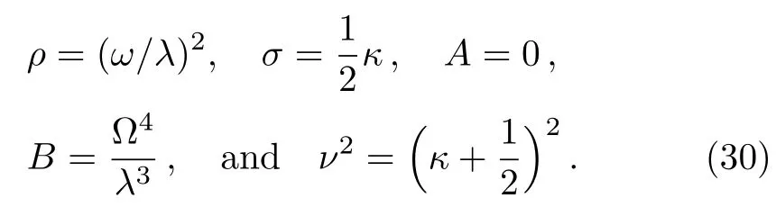
Substituting these parameters in Eq.(A7a),results in the following symmetric three-term recursion relation for the expansion coefficients of the wave function

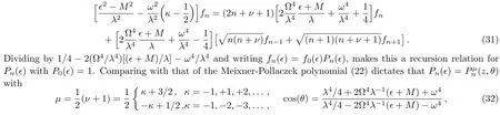
It is obvious that for positive energy whereϵ>M,these assignments violate reality sincezbecomes pure imaginary and1.Thus,we are forced to make the replacementchanging the trigonometric functions in Eq.(32)to hyperbolic and making the asymptotic wavefunction vanish since the oscillatory factor einθin Eq.(23)changes into a decaying factor e−nθ.All of this imply that there are no continuous energy scattering states but only discrete energy bound states.This,of course,is an expected result for the isotropic oscillator whose energy spectrum is con firmed using the spectrum formula of the Meixner-Pollaczek polynomial that gives

with Ω=0,this is identical to the energy spectrum of the Dirac-oscillator problem.The correspondingm-th bound state wavefunction will be written in terms of the discrete version of the Meixner-Pollaczek polynomial as

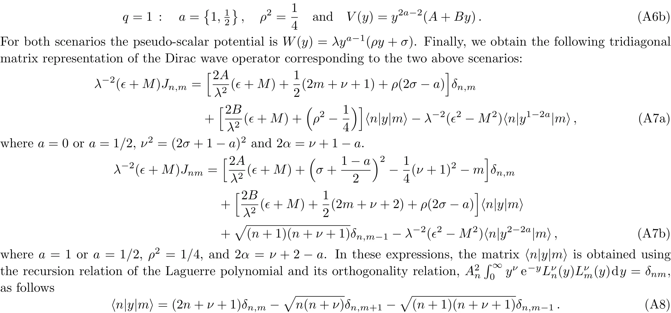
4.2 The q=1 Scenario of(A6b)

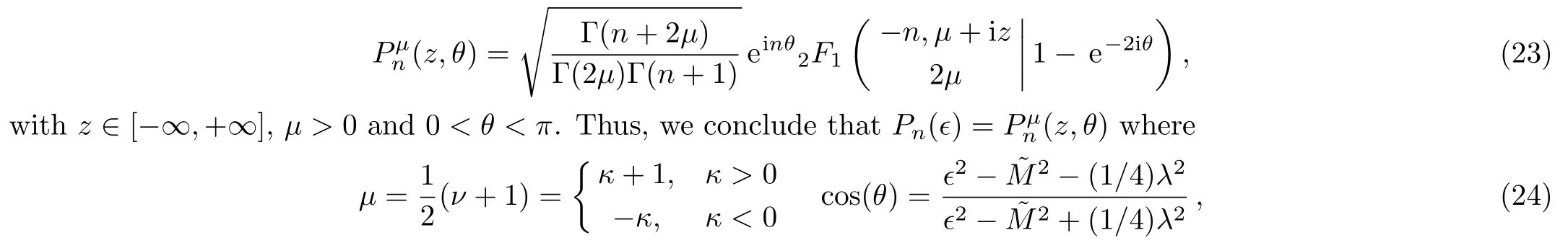
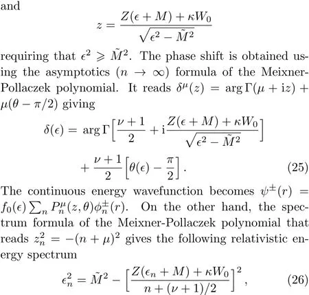
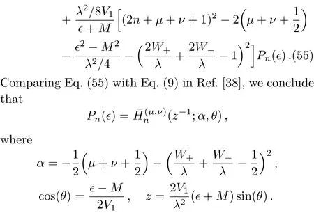
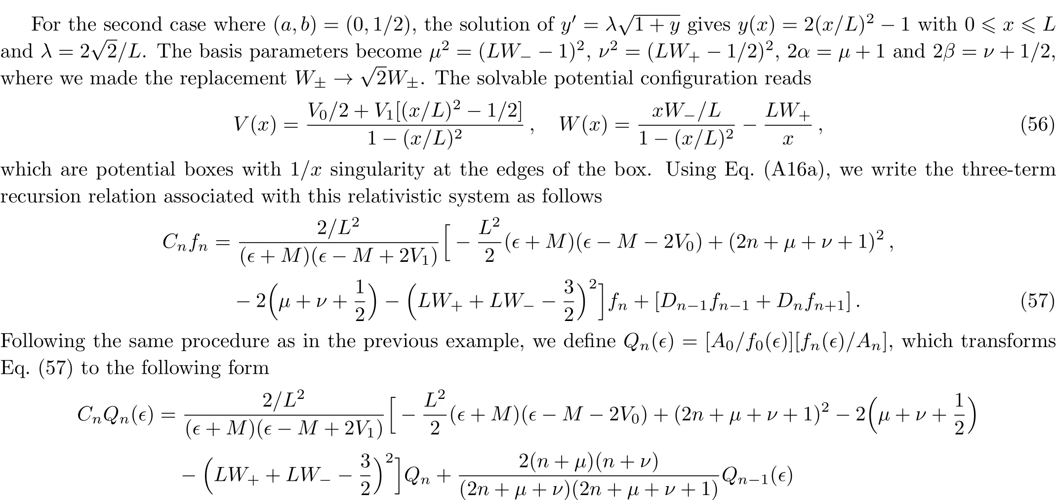
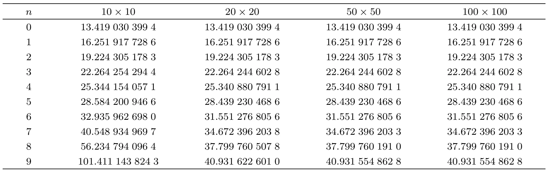
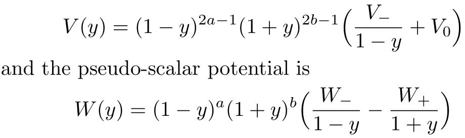
In this scenario,the vector potential isV(y) =y2a−2(A+By)and the pseudo-scalar potential isW(y)=λya−1(ρy+σ)such thatρ2=1/4.Moreover,the basis parameterνis to be determined later by physical constraints whereas 2α=ν+2−a.There are two con figurations in this scenario:one corresponds toa=1 wherey(x)=eλxwith−∞

For the first con figuration,we can write

To make the vector potential vanish at in finity we can freely chooseV0=0.Therefore,the parameters in the Dirac wave operator matrix(A7b)are as follows:

Substituting these parameters in Eq.(A7b),results in the following symmetric three-term recursion relation for the expansion coefficients of the wave function

which is a quadratic equation to be solved forϵn.WithW0=0,it is identical to the energy spectrum of the spinsymmetric Dirac-Morse problem(i.e.,with equal scalar and vector exponential potentials).Now,the continuous dual Hahn polynomial has a mix of continuous and discrete spectra forξ<0,then the following wavefunction represents the system with a mix of continuous energyϵand discrete energyϵm

5 Solution in the Jacobi Basis

Lety(x)be a coordinate transformation such that−1 6y6+1.A complete set of square integrable functions as basis in the new con figuration space with the dimensionless coordinateyhas the following elements The real dimensionless parameters{µ,ν}are greater than−1 whereas{α,β}will be determined by square integrability and the tridiagonal requirement.Substituting Eq.(50)into Eq.(6)and using the differentiation chain rule d/dx=y′(ddy),we obtain

In the following two subsections,we consider the two physical scenarios found in Appendix B and corresponding to Eqs.(A16a)and(A16b),respectively.

5.1 The(p,q)=(0,0)Scenario of(A16a)

In this scenario,the vector potential takes the formand the pseudoscalar potential reads

where we can always chooseV0=0.The vector and scalar are potential boxes with sinusoidal bottom whereas the pseudo-scalar is a potential box with 1/xsingularity of strength±2W∓at the two edges of the box.This potential con figuration was never reported in the literature.Its existence here is a demonstration of the unique advantage of the TRA over other methods for enlarging the class of exactly solvable potentials.Substituting these results back in(A16a),we obtain the following three-term recursion relation for the expansion coefficients

Some of the properties of this new polynomialwere derived numerically in Ref.[38].In contrast to the orthogonal polynomials of Sec.3,the analytical properties of this new polynomial are not yet known.Thus,the properties of the corresponding physical system(such as the phase shift and energy spectrum that would have been determined from the asymptotics of the polynomial[38])could not be given analytically or in a closed form.In the absence of these analytic properties,we give in Table 1 numerical results for the lowest part of the positive energy relativistic spectrum for a chosen set of values of the physical parameters.In Appendix C,we give the details of the procedure used in this calculation.The upper component of the spinor wavefunction is written as

The lower component of the spinor wavefunction can be easily obtained by calculatingusing Eq.(52)with

Table 1 The lowest part of the energy spectrum associated with the potential con figuration(53)for various basis sizes.We used the procedure outlined in Appendix C and took the following values of the physical parameters:M=1,λ=1,V0=0,V1=5,W+=−2,and W−=3.

Table 2 The lowest part of the energy spectrum associated with the potential con figuration(56)for various basis sizes.We took the following values of the physical parameters:M=1,L=1,V0=5,V1=−4,W+=−2,and W−=3.

5.2 The(p,q)=(1,0)Scenario of(A16b)

In this scenario,the vector potential is

whereρ=W−/λandσ=W+/λ.Moreover,the basis parameters areν2=(2W+/λ+b−1)2,2α=µ+2−a,and 2β=ν+1−b. The parameterµis fixed later by physical constraints including the( finite)number of bound states.There are three physical con figurations associated with this scenario.The first one corresponds toandx>0.The second one corresponds to(a,b)=(1/2,1/2)wherey(x)=sin(λx)and−π/2λ0.

where we have also made the replacementTo force the vector potential to vanish at in finity,we chooseV−=0. The basis parameters becomeν2=(W+/λ −1/2)2,2α=µ+1 and 2β=ν+1/2.Substituting these quantities in Eq.(A16b)and after somewhat lengthy manipulations,we obtain the following three-term recursion relation

Comparing this recursion relation with Eq.(12)in Ref.[38],giveswhereis a new orthogonal polynomial de fined in Ref.[38]withSome of the interesting properties of this polynomial are discussed in the same Ref.[38].For example,ifσis positive then this polynomial has only a continuous spectrum.However,ifσis negative then the spectrum is a mix of continuous scattering states and a finite number of discrete bound states.Moreover,the corresponding bound state energies are obtained from the following spectrum formula of the polynomial

where,again,andHowever,

which could be positive or negative depending on the sign ofTherefore,withand for negativeσthe bound state energy spectrum is obtained from the spectrum formula(61).On the other hand,for positiveσthe system has only continuum scattering states with the two-component wavefunctionand where the scattering phase shift is obtained from the asymptotics of the polynomialRn(ϵ),or equivalentlywhich is unfortunately not yet known analytically.Consequently,one needs to resort to numerical means.

6 Conclusion

In this article,we have discussed different exactly solvable potentials for the Dirac equation that have never been reported in the literature.However,we did not exhaust all possible solvable potentials in this manuscript.For example,we could have included a larger class of potentials by keepingV±̸=0 in the potentialV(x)of Subsec.5.1 pro-vided that the basis parameters become energy dependent and chosen such that

Moreover,we did not include the possibility that the basis is neither orthogonal nor tri-thogonal(i.e.,the basis overlap matrixis not tridiagonal)but the Dirac wave operator is still tridiagonal.This is accomplished by the requirement that the matrix representation of the kinetic energy operator,

contains a counter term that cancels the non-tridiagonal

We also hope that experts in orthogonal polynomials will soon derive the analytical properties of the two orthogonal polynomials mentioned in Sec.5,which will allow us to write different properties associated with the physical system in closed form,e.g.the energy spectrum and phase shift.

Appendix A The Laguerre Basis

Appendix B The Jacobi Basis

We observe a symmetry in the three scenarios above that allows us to obtain the solution corresponding to an(a,b)case by a simple parameter map from another(b,a)case.One can show that any(a,b)case belonging to Eq.(A12c)is obtained from(b,a)case in Eq.(A12b)by the following simple map

Finally,we obtain the following tridiagonal matrix representation of the Dirac wave operator corresponding to the two scenarios of Eq.(A15)above:

In these expressions,the matrixis obtained using the recursion relation of the Jacobi polynomial and its orthogonality relation,

Appendix C Energy Spectrum Calculation in the Jacobi Basis

We choose the lower component of the spinor basis to be energy independent and be related to the upper component via a relation similar to the kinetic balance equation and as follows

whereτis a non-physical computational parameter of inverse length dimension.We expect that physical results will be independent of the choice of value of this parameter as long as that choice is either unique or natural.Since the choice ofτin the formulation of the problem above isϵ+M(see below Eq.(8)),then we expect that this unique or natural choice ofτwill be different for each energy eigenvalue.If we designate the value of them-th bound state as a function ofτasϵm(τ),then the unique or natural choice ofat which

That is,the energy spectrum as a function ofτis at an extremum.In fact,the extremum condition for calculating them-th bound state energy forces the basis parameterτin Eq.(A18)to assume the value.Now,in this energy independent basis the matrix elements of the Dirac wave operator(8)become

To test the procedure,we use Eq.(A22)to calculate the energy spectra for all three problems of Subsec.5.2 and compare them to those obtained using the exact spectrum formula(61).Agreement is achieved to machine accuracy for a large enough basis size.Consequently,we employ the same procedure but using Eq.(A21)to obtain the energy spectra for the two problems of Subsec.5.1 that do not have an exact spectrum formula.Those results are shown in Tables 1 and 2.

We are honored to dedicate this work to Prof.Hashim A.Yamani on the occasion of his 71st birthday.The authors would like to thank King Fahd University of Petroleum and Minerals(KFUPM)for their support under research grant RG1502,and acknowledge the material support and encouragements of the Saudi Center for Theoretical Physics(SCTP).

[1]J.D.Bjorken and S.D.Drell,Relativistic Quantum Mechanics,McGraw-Hill,New York(1964).

[2]W.Greiner,B.Müller,and J.Rafelski,Quantum Electrodynamics of Strong Fields,Springer,Berlin(1985).

[3]W.Greiner,Relativistic Quantum Mechanics:Wave Equations,Vol.3,Springer,Berlin(1990).

[4]O.Klein,Z.Phys.53(1929)157.

[5]N.Dombey and A.Calogeracos,Phys.Rep.315(1999)41.

[6]N.Dombey,P.Kennedy,and A.Calogeracos,Phys.Rev.Lett.85(2000)1787.

[7]K.S.Novoselov,A.K.Geim,S.V.Morozov,D.Jiang,Y.Zhang,S.V.Dubonos,I.V.Grigorieva,and A.A.Firsov,Science 306(2004)666.

[8]A.De Martino,L.DellAnna,and R.Egger,Phys.Rev.Lett.98(2007)066802.

[9]A.H.Castro Neto,F.Guinea,N.M.R.Peres,K.S.Novoselov,and A.K.Geim,Rev.Mod.Phys.81(2009)109.

[10]S.Kuru,J.Negro,and L.M.Nieto,J.Phys.C 21(2009)455305.

[11]C.S.Jia,J.W.Dai,L.H.Zhang,J.Y.Liu,and X.L.Peng,Phys.Lett.A 379(2015)137.

[12]Yu Sun,G.D.Zhang,and C.S.Jia,Chem.Phys.Lett.636(2015)197.

[13]C.S.Jia and Z.W.Shui,Euro.Phys.J.A 51(2015)144.

[14]C.S.Jia,T.He,and Z.W.Shui,Comput.Theor.Chem.1108(2017)57.

[15]C.S.Jia and Y.Jia,Euro.Phys.J.D 71(2017)3.

[16]Z.W.Shui and C.S.Jia,Euro.Phys.J.Plus 132(2017)292.

[17]G.V.Shishkin and V.M.Villalba,J.Math.Phys.30(1989)2132.

[18]A.Anderson,Phys.Rev.A 43(1991)4602.

[19]G.V.Shishkin,J.Phys.A 26(1993)4135.

[20]A.V.Yurov,Phys.Lett.A 225(1997)51.

[21]C.Quesne and V.M.Tkachuk,J.Phys.A 38(2005)1747.

[22]K.Nouicer,J.Phys.A 39(2006)5125.

[23]C.Quesne and V.M.Tkachuk,SIGMA 3(2007)016.

[24]T.K.Jana and P.Roy,Phys.Lett.A 373(2009)1239.

[25]H.Akcay,Phys.Lett.A 373(2009)616.

[26]G.B.Smith and L.J.Tassie,Ann.Phys.65(1971)352.

[27]J.N.Ginocchio,Phys.Rev.Lett.78(1997)436.

[28]J.S.Bell and H.Ruegg,Nucl.Phys.B 98(1975)151.

[29]J.N.Ginocchio,A.Leviatan,Phys.Rev.Lett.87(2001)072502.

[30]J.N.Ginocchio,Phys.Rep.414(2005)165.

[31]P.Alberto,A.S.de Castro,and M.Malheiro,Phys.Rev.C 87(2013)03130.

[32]P.Alberto,A.de Castro,M.Fiolhais,R.Lisboa,and M.Malheiro,J.Phys.Conference Series 490(2014)012069.

[33]P.Alberto,M.Malheiro,T.Frederico,and A.de Castro,J.Phys.Conference Series 738(2016)012033.

[34]A.D.Alhaidari,Ann.Phys.317(2005)152.

[35]A.D.Alhaidari,J.Math.Phys.58(2017)072104.

[36]S.T.Chihara,An Introduction to Orthogonal Polynomials,Gordon and Breach,New York(1978),and references therein.

[37]R.Koekoek and R.Swarttouw,The Askey-Scheme of Hypergeometric Orthogonal Polynomials and Its q-Analogues,Reports of the Faculty of Technical Mathematics and Informatics,Number 98-17,Delft University of Technology Delft,(1998)page 37.

[38]A.D.Alhaidari,J.Math.Phys.59(2018)013503.

[39]A.D.Alhaidari,H.Bahlouli,and I.A.Assi,Phys.Lett.A 380(2016)1577.