A regional suspended load yield estimation model for ungauged watersheds

Hossein Kheirfam *,Sahar Mokarram-Kashtian

a Department of Environmental Science,Urmia Lake Research Institute,Urmia University,Urmia 57561-51818,Iran

b Department of Forestry,Tarbiat Modares University,Noor 46417-76489,Iran

Abstract Developing regional models using physiographic,climatic,and hydrologic variables is an approach to estimating suspended load yield(SLY)in ungauged watersheds.However,using all the variables might reduce the applicability of these models.Therefore,data reduction techniques(DRTs),e.g.,principal component analysis(PCA),Gamma test(GT),and stepwise regression(SR),have been used to select the most effective variables.The artificial neural network(ANN)and multiple linear regression(MLR)are also common tools for SLY modeling.We conducted this study(1)to obtain the most effective variables influencing SLY through DRTs including PCA,GT,and SR,and then,to use them as input data for ANN and MLR;and(2)to provide the best SLY models.Accordingly,we used 14 physiographic,climatic,and hydrologic parameters from 42 watersheds in the Hyrcanian forest region(in northern Iran).The most effective variables as determined through DRTs as well as the original data sets were used as the input data for ANN and MLR in order to provide an SLY model.The results indicated that the SLY models provided by ANN performed much better than the MLR models,and the GT-ANN model was the best.The determination of coefficient,relative error,root mean square error,and bias were 99.9%,26%,323 t/year,and 6 t/year in the calibration period,and 70%,43%,456 t/year,and 407 t/year in the validation period,respectively.Overall,selecting the main factors that influence SLYand using artificial intelligence tools can be useful for water resources managers to quickly determine the behavior of SLY in ungauged watersheds.

Keywords:Data reduction techniques;Forest watershed;Sediment yield;Regional models;Watershed sediment modeling

1.Introduction

The prediction of suspended load(SL)is useful in the management of rivers(Sadeghi and Kheirfam,2015).Suspended load yield(SLY)in a watershed occurs through physical processes such as soil detachment,transportation,and deposition(Yang et al.,2017).The concentration of SL depends on climatic and hydrological conditions,topography,and land cover and management strategies(Melesse et al.,2011;Cho et al.,2016;Swarnkar et al.,2018).The destruction of the Hyrcanian forests in Iran and the SL flowing from watersheds into the Caspian Sea have caused a lot of problems.Therefore,measuring and/or estimating the SLY at the watershed outlets aids in management decisions(Kis‚i,2010).Despite the need to obtain accurate estimates of SLY at the watershed outlets,due to their large values,establishing SLY measurement stations in all Hyrcanian forest watersheds is not possible or economical.For this reason,it is necessary to estimate and predict SLY.Although the estimation of SLY is often conducted with rating curves(Tramblay et al.,2010),these models have a high estimation error for SLY regional analyses(Asselman,2000).Tramblay et al.(2008)indicated that the correlation between the annual maximum SLY and discharge was significant at only 92 stations out of 208 stations in North America.In this regard,Swarnkar et al.(2018)found that SLY varied with morphoclimatic regimes of watersheds,and Choubin et al.(2018)also reported the high variability of SLY induced by hydro-meteorological regimes for the watersheds of the north of Iran.Accordingly,in addition to discharge,various variables can be used to estimate the magnitude of extreme SLY,including topography,land cover,and climatic properties(Jarvie et al.,2002;Restrepo et al.,2006;Tramblay et al.,2008;Nadal-Romero et al.,2014;Swarnkar et al.,2018).It is necessary to investigate the efficiency of using climatic,hydrologic,and physical characteristics of watersheds for SLY modeling in ungauged watersheds with SLY measurement stations(Caratti et al.,2004).The extension of those models to watersheds lacking SLY measurement stations could be a convenient and practical approach(Tramblay et al.,2010).

Nevertheless,a large number of input variables is one of the most common limitations of this modeling process(Cruz-C´ardenas et al.,2016).Therefore,it is recommended to reduce the number of input variables through data reduction techniques(DRTs)(Lin and Wang,2006;Noori et al.,2011).Although various techniques are used to reduce the number of input variables,they have different mechanisms,processes,and capabilities.Therefore,it is necessary to select an appropriate DRT to obtain an optimum mode with consideration of the intended use case.For hydrological modeling,principal component analysis(PCA)(Ouarda et al.,2006;Zhang,2007),Gamma test(GT)(Corcoran et al.,2003;Moghaddamnia et al.,2009),and stepwise regression(SR)(Noori et al.,2010;Vanmaercke et al.,2011)are widely used.The above-mentioned DRTs have been used to predict discharge, flooding, evaporation, and water quality(Ramachandra Rao and Srinivas,2006;Robertson et al.,2006;Khan et al.,2007;Rashidi et al.,2016;Mohammadi et al.,2018;Sharifi Garmdareh et al.,2018),individually.Although these techniques have also been widely used to estimate river f l ows and/or SLY,there is not yet a reference technique for developing accurate models,though in one case,Kakaei-Lafdani et al.(2013)estimated the daily SLY using DRTs(GT and genetic algorithm)and predictor softwares(artificial neural network(ANN)and support vector machine).

It is obvious that the selected and introduced input data from various techniques may differ from one another,leading to different results of SLY estimation,and thus,leading to miss-managements of watersheds.Therefore,it is important for us to use the most appropriate and accurate technique(s)to select the most effective variables and then use them in SLY estimation models.In addition to using suitable DRTs,it is essential to apply accurate and user-friendly models to SLY estimation.To this end,many models have been used to estimate SLY.Of the most widely used techniques,the ANN and multiple linear regression(MLR)techniques are most often recommended due to their high accuracy and user-friendliness(Kis‚i,2008;Rajaee et al.,2011;Zare Abyaneh,2014;Nourani and Andalib,2015;Samantaray and Ghose,2018).However,for accurate SLYestimation,the ANN models are preferred to the MLR models(Yilmaz et al.,2018).In addition,Khan et al.(2016)successfully used the ANN to model hydrodynamic components of the Ramganga River Catchment of the Ganga Basin,India,an ungauged region with unreachable terrain.By and large,we need a comprehensive assessment to introduce accurate,applicable,and user-friendly model(s)for SLY estimation in ungauged watersheds.To this end,in this study we attempted to provide an appropriate regional model for SLY estimation in ungauged watersheds using input variable reduction techniques such as PCA,GT,and SR,as well as using ANN and MLR tools for modeling.

2.Materials and methods

2.1.Watershed characteristics and data collection

In this study,we selected the Hyrcanian forest watersheds,located south of the Caspian Sea,as the study area due to the importance of its regional environment.The watersheds that are located upstream of the Lahijan-Nour,Haraz-Neka,and Gorganroud rivers were selected for this research(Fig.1).The Lahijan-Nour and Haraz-Neka rivers are located at longitude 49°48′E to 54°41′E and latitude 35°36′N to 37°19′N,covering an area of approximately 28463 km2.The Gorganroud Watershed is located southeast of the Caspian Sea at longitude 54°02′E to 56°16′E and latitude 36°34′N to 37°47′N,covering an area of 13170 km2.The climate of this watershed is semiarid to semi-humid(Kheirfam and Vafakhah,2015).Additionally,the mean annual temperature of all the watersheds varies from 16.7°C to 19.1°C across the study area from the west to the east.The study area is also a part of the South Caspian Depression,which is bordered to the south by the Elburs mountainous system and to the north by the Caspian Sea.The Gilan,Mazandaran,and Golestan plains are located in the western,central,and eastern parts,respectively.This region represents the Elburs foredeep, filled with a thick sequence of Neogene-Quaternary sediments and separated from the Elburs fold system by a deep-seated regional fault(Svitoch et al.,2013).Other properties of the study area are presented in Table 1.

Our raw data were obtained from Kheirfam and Vafakhah(2015).Fourty-two watersheds were selected for the SLY modeling process using 14 climatic,hydrologic,and physiographic variables(Table 1).Furthermore,we used the SLY data obtained from the Iran Water Resources Management Company(IWRMC),which were calculated with the sediment-rating curve(SRC)function.

Fig.1.Overview of study region and location of selected watersheds.

Table 1 Definitions and characteristics of variables for study watersheds.

2.2.Input variable reduction

As mentioned above,in order to achieve the best SLY model,we used three DRTs to select the variables with the most significant influence on SLY in the Hyrcanian forest watersheds,including SR(Faraway,2002;Bethea,2018),PCA(Abrahams,1972;White,1975;Hess and Hess,2018),and GT(Koncar,1997;Adoalbj¨orn et al.,1997;Liu et al.,2003;Mohammadi et al.,2018).SR is a general statistical method and a combination of forward and backward methods that use the step-by-step algorithm to select the most effective variables based on the linear regression model.After adding all independent variables one by one,they are sorted according to their correlation coefficients(R)with the output variable.The variables with optimumRvalues are selected as the model input variables(Sharma and Yu,2015).PCA is widely used to identify the most effective variables from among the large number of variables.Due to this,the linear correlation between two or more variables can be established.Then the variables are summarized in a scatter plot,which is called the factor load.After this,the most effective variable influencing SLY is identified,and additional lines are drawn to maximize the remaining variability in a consecutive step-by-step extraction of factors.The variables with the highest factor loadings within each separate factor will probably share a common characteristic or combination of characteristics.The efficiency of the PCA method has been validated using Kaiser-Meyer-Olkin(KMO)and Bartlett tests(Shrestha and Kazama,2007;Peres and Fogliatto,2018).GT is another DRT that can be achieved through the use of the winGamma TM software.To identify the most effective variable(s),all the input variables are uploaded to the software first.Then,one of the variables is eliminated from the main set and the Gamma value of this run is recorded.In the second run,the eliminated variable in the first run is added to the main set,and the second variable will be eliminated.These runs are done for all the variables respectively and the Gamma values are recorded each time.Finally,the variables with the highest Gamma values,which are recorded through a procedure of elimination,are selected as input variables.Unlike SR and PCA,GT is a nonlinear technique(Moghaddamnia et al.,2009).More detailed methodological and functional descriptions of these techniques were expressed in our previous research(Kheirfam and Vafakhah,2015).

2.3.SLY modeling techniques

2.3.1.ANN

The ANN,designed by McCulloch and Pitts(1943),has been widely used as a forecasting tool in natural sciences.It might be one of the most successful technologies in the last two decades.The ANN has an input layer,a hidden layer,and an output layer.Each layer is made up of several nodes,and layers are interconnected by sets of correlation weights.In order to conduct the sediment prediction,the multi-layer perceptron(MLP)network has been recommended for different types of ANN(Kis‚i,2010;Heng and Suetsugi,2013).Also,in natural sciences modeling with the ANN,the feed forward(FF)and the back-propagation(BP)algorithms are common training process methods.However,it has been proven that the BP algorithms have the best performance in hydrological modeling(Maier and Dandy,1999;Nourani and Andalib,2015;Khan et al.,2016).Each node in an ANN layer receives and processes a weighted input from a preceding layer and transmits its output to nodes in the following layer through links(Vafakhah et al.,2014).The link equations and their description can be found in Khosrobeigi-Bozchaloei and Vafakhah(2015).We used four data sets,which were obtained from PCA,GT,and SR techniques,as well as raw data sets(all the 14 variables),to estimate SLY in the studied watersheds.Then,the SLY data were normalized to prevent attributes or features in greater numerical ranges from dominating those in smaller numerical ranges,as well as numerical difficulties during the calculation.In the modeling process,the data sets of SLY were scaled to a range between-1 and 1.Also,the Levenberg-Marquardt(LM)algorithm was applied to the training stage in the ANN model(Hagan and Menhaj,1994).Sigmoid tangent and linear activations were used for the hidden layer and output layer nodes,respectively(Vafakhah et al.,2014).The number of the hidden layer nodes of each model was determined after trying various network structures.The ANN training was stopped after 1000 iterations.

2.3.2.MLR

MLR,as a statistical method,is one of the suitable tools for modeling the linear relationship between a dependent and one or more independent variables of small sample size(Razi and Athappilly,2005).MLR attempts to model the relationship between two or more explanatory variables and a response variable by fitting a linear equation to the observed data(Bethea,2018).Each value of the independent variable(X)is associated with a value of the dependent variable(Y).As in the ANN modeling process,four data sets that were obtained from PCA,SR,and GT variable reduction results as well as the original data set were used as separate input data sets for the SLY modeling by MLR.

2.4.Model performance evaluation

In order to evaluate the performance of the regional SLY estimation models provided,80%of the watersheds were used randomly for the calibration(training)period and the remaining 20%of the watersheds were used for the validation(testing)period.Then,the models were evaluated using the relative error(RE),root mean square error(RMSE),determination of coefficient(R2),and bias(BIAS)as follows:

whereOsiandMsiare theith observed and estimated mean annual SLY,respectively;OmandMmare the average values ofOsiandMsi,respectively;andNis the number of observed data.

3.Results and discussion

3.1.Most effective variables

In this study,the KMO value and the significance level of Bartlett's test for the PCA technique were 0.775 and 520.48,respectively.Therefore,PCA was considered a suitable technique for selecting the most effective variables for SLY modeling in the Hyrcanian forest watersheds according to Shrestha and Kazama(2007).Through the PCA process,we found that of the 14 variables the following five were the most effective,which explained 82.63%of variability:Sl(45.74%of variability),Q2(12.02%of variability),Hw(9.89%of variability),A(7.66%of variability),andPr(7.32%of variability).

Along with PCA,we determined the most important variables using the GT technique,a nonlinear method,according to the observed minimumREresults(Tsui et al.,2002).Noori et al.(2010),also using the GT technique,distinguished the influence values of variables with a one-to-one removing replacing strategy.The results of this process,in which all variables were repeated individually,indicated thatQp(with a Gamma value ofGv=0.61746),Ff(withGv=0.13562),Ss(withGv=0.13546),Lw(withGv=0.13328),andCc(withGv=0.13271)were the most effective variables in SLY modeling.

In addition to PCA and GT,the SR technique was also used as a linear method(Amendola et al.,2017)to select the important variables for modeling the SLY in the studied watersheds based on theirR2results.Accordingly,we used the stepwise method from regression models,in which the variables were input individually,and this operation continued until the error reached the desired significance level(Durrant,2001).The results showed thatQpandQ2were distinguished as the most effective factors.

Our results indicated thatQpandQ2were the most effective watershed variables that had the most significant influence on the SLY in the Hyrcanian forest regions.The SLY was supplied by wash loads(with diameters of less than 63 μm,yielded from the watershed area)and bed material loads(with diameters of greater than 63 μm,yielded from the river bed and bank)(Sadeghi and Zakeri,2015).In the forest watersheds,the contribution of wash loads to SLY was negligible(Sadeghi and Kheirfam,2015;Kheirfam and Sadeghi,2017).Therefore,the major portion of SLY was supplied from bed material loads(Sadeghi and Zakeri,2015).Bed material loads mostly varied with the river flow variation(e.g.,QpandQ2).In this regard,previous studies(Lobera et al.,2016;Rainato et al.,2017;Ebabu et al.,2018)indicated that the major volume of annual and daily suspended sediment transported byQpandQ2,respectively,confirmed the decisive role of these variables.However,human intervention (eg., deforestation, land use change, overexploitation,and land degradation)has led to the decrease of the Hyrcanian watershed cover.During rain events,the wash load share in SLY increases(Sadeghi and Kheirfam,2015).In this study,Prwas selected(by GT)as one of the important factors.Additionally,some physical variables of watersheds(Hw,A,Ff,Ss,Lw,andCc)were also distinguished through the PCA and GT techniques as effective variables influencing SLY.However,indirectly,these variables also influenced the river's hydrological behavior and the SLY(Bywater-Reyes et al.,2017).

3.2.Regional SLY estimation modeling

After selecting the most important variable using PCA,SR,and GT,the ANN and MRL were used to provide regional SLY models separately for each data set.Then,the statistical criteria were used to evaluate the performance of provided models and also to select and introduce the most appropriate regional SLY model.The structures of ANN and MLR models are given in Table 2,and the results of the evaluation performance by statistical criteria are provided in Tables 3 and 4.

According to Table 3 and statistical analyses,the minimum,maximum,average,standard deviation,and coefficient of variation of input data in the calibration period were 112 t/year,89440 t/year,3900 t/year,and 14793 t/year,and 379%,respectively.These statistical criteria can provide useful information about the accuracy or errors of the provided models.In the calibration period,the MLR models could not estimate low values of SLY,as they underestimated the low values of observed SLY.In the validation period,we also observed the underestimated results from the MLR models for low values of SLY.In this regard,Kutner et al.(2004)reported that the MLR models describe a linear relationship between variables,and therefore,imbalance in the higher and lower values of the SLY data leads to overestimated and underestimated results from MLR models(McNeish and Stapleton,2016),similar to our data set.Meanwhile,in the calibration period for the ANN models,the estimated low values of SLY were very close to the observed values.However,the estimated low values of SLY in the validation period were acceptable.Unlike the storm events,the low values of SLY only depended on the low flow events(Sadeghi and Zakeri,2015;Sadeghi et al.,2018).Therefore,the ANN models easily simulated the low values of SLY that have a good fitting with water flow(Talebizadeh et al.,2010).In contrast to this,in the storm events,different nonlinear relationships governing the process of soil detachment and final SLY(Sadeghi and Zakeri,2015;Swarnkar et al.,2018)might lead to the inability of the ANN models to estimate high SLY values.The ability of the ANN models to precisely estimate low SLY values has been reported(Talebizadeh et al.,2010).

In the meantime,for low values of SLY,the SR-ANN and PCA-ANN models had the best estimation of SLY in the calibration period,and for the original data set(ORG),the ANN model had the best SLY estimation during the validation period by 113,113,and 408 t/year,respectively(Tables 3 and 4).For high values for the calibration period,the MLR models underestimated the SLY.However,they had acceptable results.The analyses of the other statistical criteria indicated that the values of bias criteria for the ORG-MLR,SR-MLR,PCA-MLR,and GT-MLR models were 7.46,0.17,8.40,and 0.03 t/year,respectively,during the calibration period(Table 3).The variables selected by PCA(Sl,Q2,Hw,A,andPr)increased the bias of MLR results,which might be related to thePreffects on the SLY results.As described earlier,the SLY behavior became significantly more complicated with precipitation(or storm events). Therefore,it did not follow a systematic trend(Gao et al.,2013).This caused confusion in the PCA-MLR model.Regarding the SR-MLR model,selectingQ2andQpas the most effective variables led to low-bias estimation results due to the high dependence of SLY on the water flow,unlike the storm events.In addition to flow components(Q2andQp),using the physiographic parameters of watersheds(Ff,Ss,Lw,andCc)as non-variable properties can also improve the ability of the models in SLY estimation(Chen,2018).We selected these parameters with the GT technique for GT-MLR modeling.

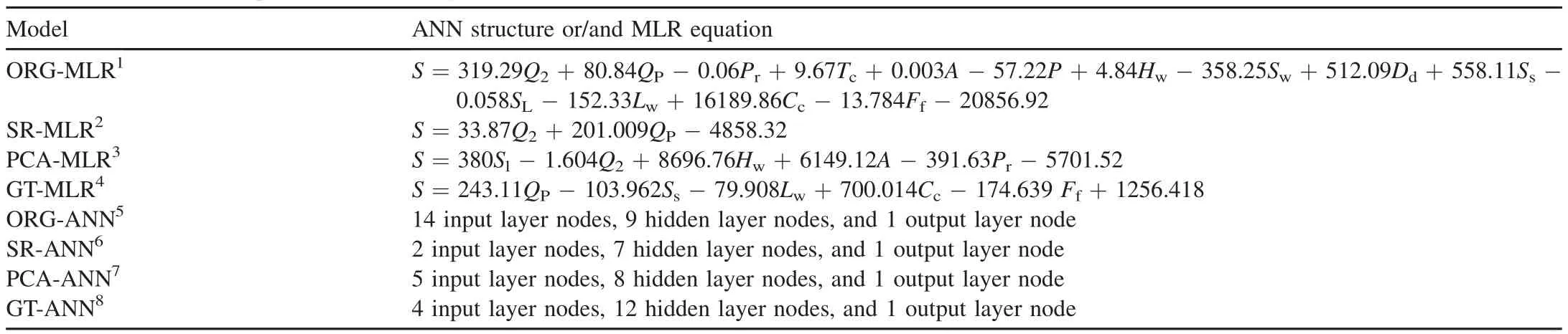
Table 2 Structures of ANN and equations of MLR regional SLY estimation models.

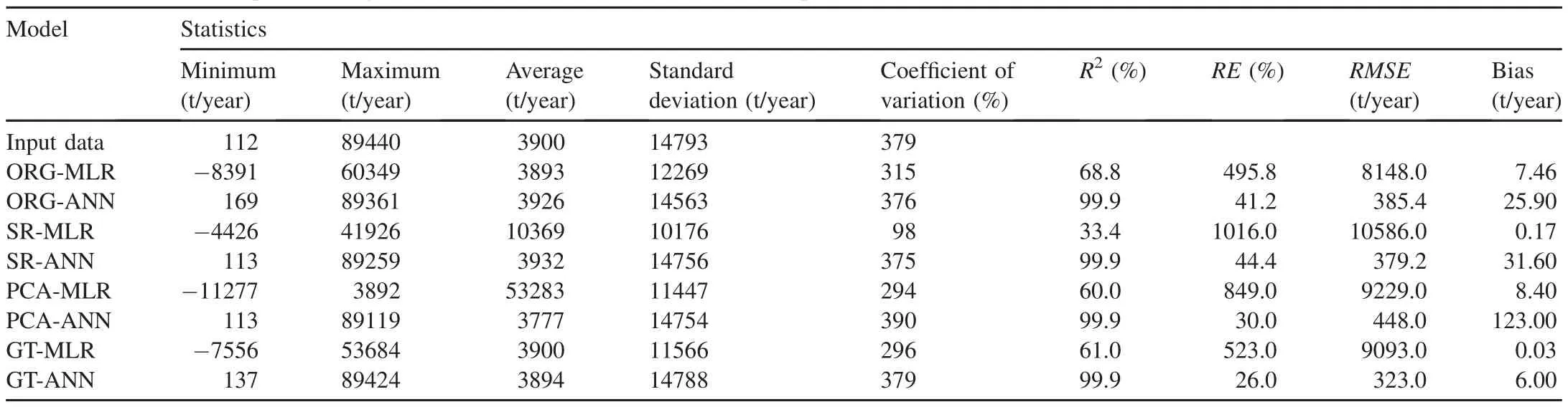
Table 3 Summarized statistics of provided regional SLY estimation models in calibration period.

Table 4 Summarized statistics of provided regional SLY estimation models in validation period.

According to the evaluation of regional SLY estimation models shown in Tables 3 and 4,the performance of the ANN models was better than that of the MLR models in both the calibration and validation periods.However,compared to the MRL models,the superiority of the ANN models was proven when estimating daily SLY(Melesse et al.,2011;Pektas and Cigizoglu,2017).Of the ANN models,the GT-ANN model was the best for regional SLY estimation.The values ofR2,RE,RMSE,andBIASfor the calibration and validation periods were 99.9%,26%,323 t/year,and 6 t/year;and 70%,43%,456 t/year,and 407 t/year,respectively.However,the PCAANN,SR-ANN,and ORG-ANN models also had acceptable estimation results.However,the large number of input data requirements was a major limitation for the ORG-ANN model.As various studies(Noori et al.,2011;Kakaei-Lafdani et al.,2013;Kheirfam and Vafakhah,2015;Mohammadi et al.,2018;Sharifi Garmdareh et al.,2018)have confirmed,the pre-processing of the most effective input variables improves the accuracy of black and/or gray box models,which is consistent with the present study.In contrast to PCA and SR,GT was a nonlinear valuator for rating the variables according to their effectiveness on the dependent variable(Chang and Heinemann,2018).Thus,it has a high capability of evaluating a high-volatility data set(e.g.,SLY).The fitting of the estimated and observed SLY values by all of the models is presented in Figs.2-5.According to these figures,the best fitting results were observed in the ANN models,particularly with the combination of the GT and PCA techniques.

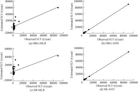
Fig.2.Fitting of estimated and observed SLY values by ORG-MLR,ORG-ANN,SR-MLR,and SR-ANN models in calibration period.

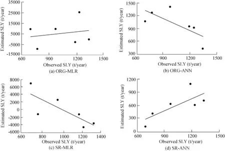
Fig.3.Fitting of estimated and observed SLY values by ORG-MLR,ORG-ANN,SR-MLR,and SR-ANN models in validation period.

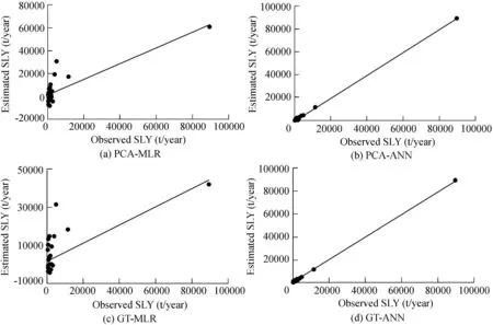
Fig.4.Fitting of estimated and observed SLY values by PCA-MLR,PCA-ANN,GT-MLR,and GT-ANN models in calibration period.

4.Conclusions

(1)Of the DRTs,GT had the best performance in selecting the most effective input variables for both the ANN and MLR models in the SLY estimation.

(2)Of all the variables,Q2andQphad the most significant effect on the SLY in the Hyrcanian forest watersheds.

(3)Overall,the ANN models performed better than the MRL models in the SLY estimation.

(4)We found that the GT-ANN model had the best performance in estimating the regional SLY.Therefore,it can be considered an economic,appropriate,and reliable approach for estimating the SLY in ungauged watersheds.

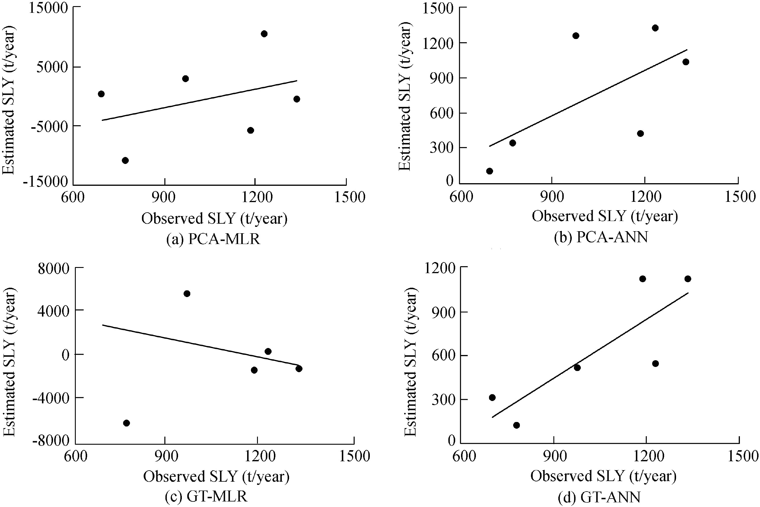
Fig.5.Fitting of estimated and observed SLY values by PCA-MLR,PCA-ANN,GT-MLR,and GT-ANN models in validation period.

(5)The MLR models considered the deviation of the final estimated and observed results in order to achieve the best estimation for the overall data set(an average),which caused the poor estimation for the one-to-one data.In ANN,on the other hand,using the iteration method to train the model led to accurate estimation for both the one-to-one and the overall data sets.

(6)For future research,we recommend using a large number of data sets to develop reliable models.Using other data reduction techniques and modeling methods(e.g.,adaptive neuro-fuzzy inference,support vector machines(SVM),and neuro-fuzzy systems)could lead to a more complete awareness of the capabilities of the models.

Acknowledgements

We would like to thank Dr.Mehdi Vafakhah,Dr.Akbar Najafi,Eng.Alireza Motevalli,Eng.Saeid Janizadeh,and Eng.Saeid Khosrobeigi Bozchaloei for their valuable assistance during different stages of this study.