Free-surface long wave propagation over linear and parabolic transition shelves

Ikh Mgdlen ,Irynto ,Dominic E.Reeve *

a Faculty of Mathematics and Natural Sciences,Bandung Institute of Technology,Bandung 40132,Indonesia

b Informatics Department,Indramayu State Polytechnic,Indramayu 45252,Indonesia

c College of Engineering,Swansea University,Bay Campus,Swansea SA2 8PP,UK

Abstract Long-period waves pose a threat to coastal communities as they propagate from deep ocean to shallow coastal waters.At the coastline,such waves have a greater height and longer period in comparison with local storm waves,and can cause severe inundation and damage.In this study,we considered linear long waves in a two-dimensional(vertical-horizontal)domain propagating towards a shoreline over a shallowing shelf.New solutions to the linear shallow water equations were found,through the separation of variables,for two forms of transition shelf morphology:deep water and shallow coastal water horizontal shelves connected by linear and parabolic transition,respectively.Expressions for the transmission and reflection coefficients are presented for each case.The analytical solutions were used to test the results from a novel computational scheme,which was then applied to extending the existing results relating to the reflected and transmitted components of an incident wave.The solutions and computational package provide new tools for coastal managers to formulate improved defence and risk mitigation strategies.

Keywords:Shallow water equation;Long-period wave;Shoaling;Analytical solution;Numerical solution;Reflection coefficient;Transmission coefficient

1.Introduction

Deep water waves can undergo dramatic changes as they propagate towards a shoreline over an irregular seabed.The processes of refraction,shoaling,diffraction,and breaking can significantly alter wave heights and directions near the shore,and must be adequately accounted for in developing beach protection and flood defence.The wave period is also an important parameter in the design of coastal structures,particularly in relation to the process of shoaling.Long-period waves,such as tsunamis,storm surges,and swells,have greater wave lengths than local storm waves,and are therefore more susceptible to the effects of shoaling.Shoaling in particular can lead to reductions in wave length and speed,as well as amplification of wave height.As long waves propagate into the coastal zone over a shelving seabed,some of the wave energy will be reflected and some will be transmitted shoreward.The focus of this paper is on wave shoaling,as well as the transmission and reflection coefficients.

This topic has been the subject of extensive research through experiments,analytical methods,and numerical modeling.Approaches can be categorized broadly into the following three categories:two horizontal dimensions(2DH);vertical slices(2DV);and resolving the vertical and horizontal structures of the wave field(3D).Early analytical treatments,such as those of Carrier(1966)and Synolakis(1987),were 2DVand focused on predicting the run-up level of long waves.These have been supplemented by other analytical solutions accounting for refraction and friction(Nielson,1983,1984)and cnoidal wave theories such as those in Sadeghian and Peyman(2012).A wide range of 2DV computational models have been developed and are based predominantly on the Boussinesq equations,the shallow water equations,or Reynolds-averaged Navier-Stokes (RANS) formulations.RANS modeling is the most computationally expensive of these equations and for that reason is limited to describing waves in a small domain such as the surf zone(e.g.,Lin and Liu,1998).There are comparatively fewer computational requirements for solving the Boussinesq equations.As a consequence,various forms of Boussinesq equations have been developed for both 2DV and 2DH applications.Early attempts were able to capture some nonlinear effects but encountered difficulties with accurate representation of linear dispersion properties at all water depths(e.g.,Nwogu,1993).More recent developments have allowed this deficiency to be addressed,at the cost of additional complexity(e.g.,Madsen et al.,2002).

Early 2DH wave models were based on a form of the elliptic mild slope equation proposed by Berkhoff(1972),which account for refraction and diffraction and provide the variation of wave amplitude over a 2DH spatial domain.A more general time-dependent form was subsequently proposed by Smith and Sprinks(1975).The computational challenges of solving an elliptical wave equation led to the development of various parabolic approximations,such as those in Radder(1979),Kirby(1986),Ebersole(1985),and Panchang et al.(1988),as well as methods for solving the transient problem via a hyperbolic formulation(Copeland,1985).An efficient means of solving the elliptic mild slope equation was proposed by Li and Anastasiou(1992),and extended by Li et al.(1993)to treat irregular wave propagation.Further developments of this theme have seen the inclusion of nonlinear effects by Beji and Nadoaka(1997);description of the wave field through an angular spectrum by Dalrymple et al.(1989),Suh et al.(1990),and Reeve(1992);and alternative derivations by Kim et al.(2009).

Here,we considered long waves occurring on a shelving foreshore and used the shallow water equations(SWEs)in a 2DV domain.Bautista et al.(2011)derived an analytical solution for long wave propagation over a linear transition shelf using a singular perturbation analysis based on the Wentzel-Kramers-Brillouin(WKB)technique.In this study,we derived analytical solutions to the linear SWEs based on the variable separation method and also developed a staggered finite volume method for their numerical solution.

This paper is organized as follows:Section 2 contains a brief description of the SWEs for waves propagating over linear and parabolic transition topography,and analytical solutions for the wave reflection and transmission coefficients are derived using the variable separation method,leading to solutions in terms of Bessel functions and polynomials;a staggered finite volume method for solving the SWEs over arbitrary topography is presented in Section 3;and in Section 4,we describe the implementation of our scheme to simulate wave propagation over linear and parabolic transition shelves.Moreover,to validate the numerical model,the computational solutions are compared with the analytical solutions and other results from previous studies.The validated numerical model is then applied to a topographic transect of the coast of Aceh,Indonesia.Conclusions are presented in the final section.

2.Shallow water model

2.1.Background

In this study,we considered a layer of ideal fluid,bounded above by a free surface and below by an impermeable bottom topographyz=-h（x）,wherex,z,andhare independent variables denoting the horizontal direction,vertical direction,and water depth,respectively.The following shallow water model for long waves in a relatively shallow region was adopted,following Kowalik(1993):

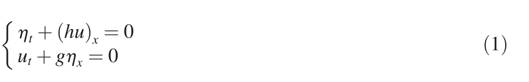
whereuis the horizontal velocity,η is the free surface elevation measured from the still water level,gis the gravitational acceleration,andtis time.Eq.(1)represents the conservation of mass and momentum balance.The physical domain considered is shown in Fig.1.

The physical domain is divided into three different regions:Ω1, Ω2,and Ω3,with prescribed depths defined by the following relationships:

(1)Linear transition shelf:

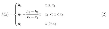
wherex1andx2are the locations of the left and right borders of the second domain,respectively;andh2andh3are the depths in the first and third domains,respectively.For the linear transition shelf,we assumed thatx1=0 andx2=L,whereLis the horizontal extent of the sloping bottom.

Fig.1.Definition of model domain.

(2)Parabolic transition shelf:

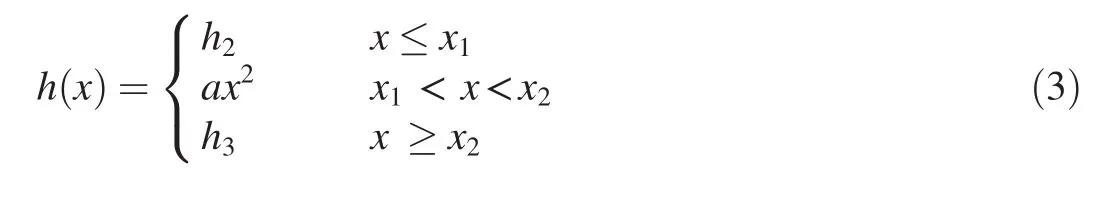
whereh2=,h3=andais an arbitrary parameter.

In the following two subsections,we derive the reflection and transmission coefficients of the free surface over the linear and parabolic transition shelves,respectively.When waves propagate over a shelf,they undergo a scattering process,with some of the wave energy being transmitted shoreward and some reflected back towards the deep sea.Analytical solutions of the SWEs can be derived based on multiple-scale asymptotic expansion(Mei et al.,2005;Noviantri and Pudjaprasetya,2010)and the well-known WKB perturbation techniques(Bender and Orszag,1978;Bautista et al.,2011).Here,solutions of the linear SWEs are derived using the variable separation method.

2.2.Reflected and transmitted waves for linear transition shelf

In domain Ω1the seabed is flat and the governing equations are as follows:

Using the variable separation method,the general solutions of η（x，t）andu（x，t）in domain Ω1are written for a monochromatic wave with unknown spatial dependence,F（x）andG（x）,and arbitrary frequency ω:

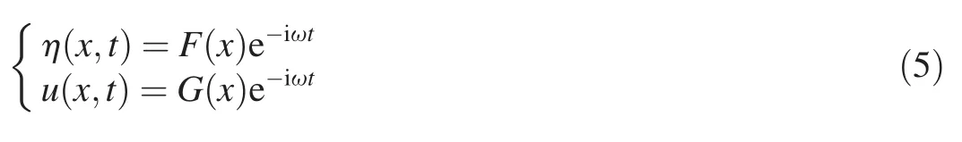
Substituting Eq.(5)into Eq.(4)yields the following:

whereaiis the amplitude of the incoming wave,andaris the amplitude of the reflected wave.The wave number,k0,in domain Ω1obeys the following dispersion relation:

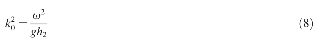
Next,substituting Eq.(7)into Eq.(5)yields the following expressions for the free surface and velocity:

In domain Ω2the governing equations for the linear transition region become

As in domain Ω1,a general solution in the form given in Eq.(5)is sought.Substituting Eq.(5)into Eq.(10)yields

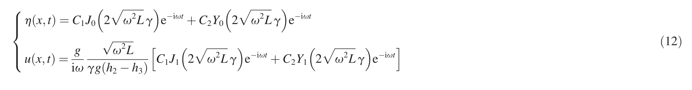
With the solution ofF（x）,and by differentiatingF（x）with respect toxand substituting the resultinto Eq.(6),the solutions to Eq.(6)are obtained:

whereJ1andY1are the first-order Bessel functions of the first and second kinds,respectively.

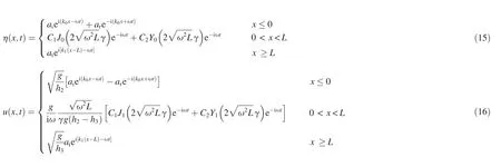
Considering an incoming wave from the deep-waterarea with depthh2propagating shoreward,the wave is partially reflected and partially transmitted while passing through the linear transition shelf.In the nearshore region Ω3,where the water depth is shallow,there is only a transmitted wave(propagating to the right,as shown in Fig.1),with an amplitudeat,and the solution is given by

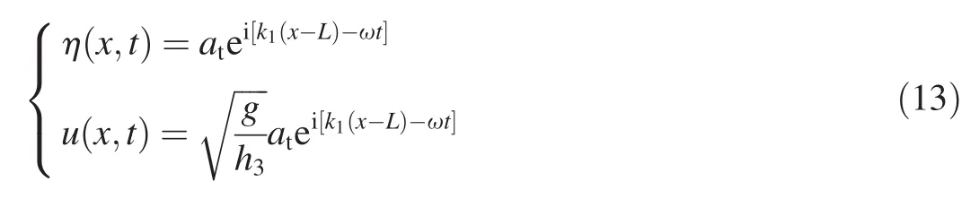
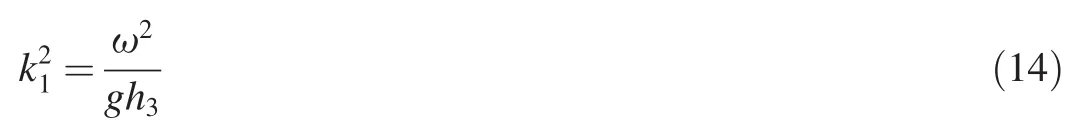
wherek1obeys the following dispersion relation:

In general,accounting for the transmitted and reflected parts of the incident wave train,the free surface η（x，t）and horizontal velocityu（x，t）throughout the domain can be formulated as follows:

with

The solution of the equations above is x=A-1b.This leads to the wave reflection and transmission coefficients that are respectively defined as

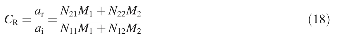
At the pointsx=0 andx=L,where the three regions connect,matching conditions must be used to conserve the free surface and horizontal momentum across the whole domain.There are,therefore,four equations with four unknown variables in the matrix form,which may be written as Ax=b,where

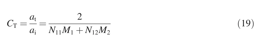
whereN11,N12,N21,N22,M1,andM2are defined as follows:

Explicit expressions for the coefficientsC1andC2are given in the matrix x in Eq.(17).

2.3.Reflected and transmitted waves for parabolic transition shelf

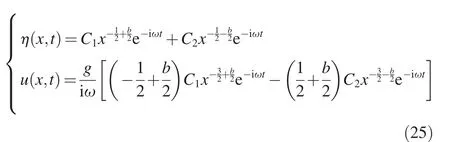
Approaches similar to those explained in Subsection 2.2 are used to find the wave reflection and transmission coefficients for a parabolic transition shelf.The free surface elevation and horizontal velocity in domains Ω1and Ω3are expressed as follows:

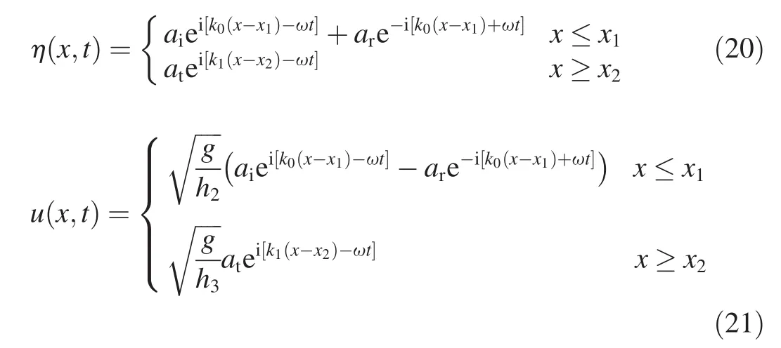
In domain Ω2,the governing equations for the shelf with parabolic transition topographyh（x）=ax2read as follows:

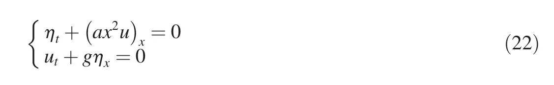
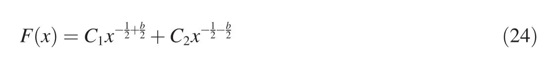
These equations may be solved within domain Ω2in exactly the same manner as before.Seeking solutions of η（x，t）andu（x，t）of the form given in Eq.(5)and substituting the results into Eq.(22)yield

The solution ofF（x）in Eq.(23)is

The matching conditions are also used to conserve the free surface η（x，t）and the horizontal momentumh（x）u（x，t）along the discontinuity points,x=x1andx=x2,which give us four equations with four unknown variables,ar,at,C1,andC2.By determiningarandatand the coefficientsC1andC2,we obtain the following reflection and transmission coefficients for wave propagation over a parabolic transition shelf:

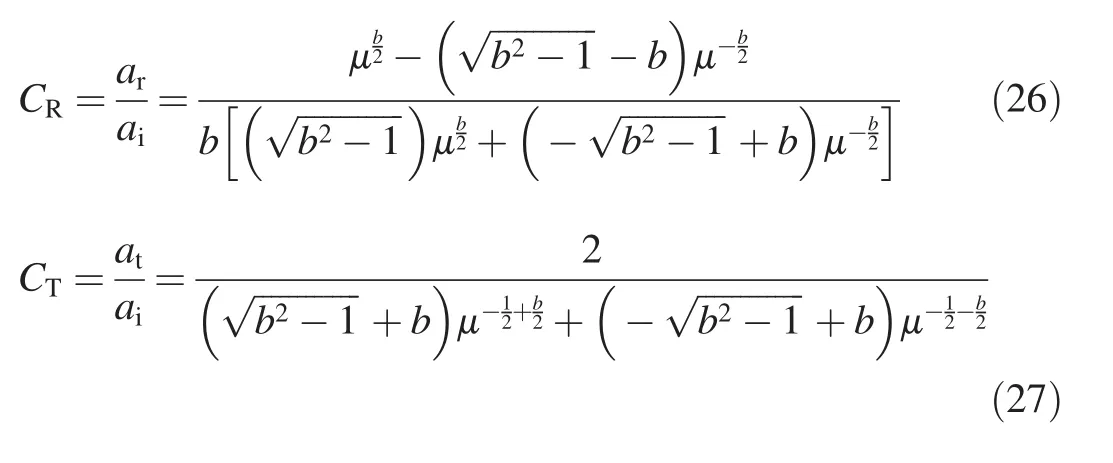
where μ=x1/x2.

For the linear transition case,Fig.2(a)and(b)shows the variations ofCRwithLandh2/h3,respectively,and Fig.2(c)and(d)shows the variations ofCTwithLandh2/h3,respectively.CRandCTare virtually independent ofLfor the range 1 m＜L＜10 m.CRrises ash2/h3increases to about 3.5,and then decreases slightly ash2/h3increases further.In contrast,CTrises monotonically withh2/h3.

Corresponding results forCRandCT,as functions of ω2/（ga）,for the parabolic transition case are shown in Fig.3(a)and(b).The trend is thatCTincreases with ω2/（ga）,μ,andh2/h3,meaning that more wave energy propagates towards the coast with the increases of ω2/（ga）,μ,andh2/h3.Fig.4 shows thatCT,as a function ofh2/h3,exhibits similar variations for both the parabolic and linear transition cases,which is also in close agreement with the analytical result of Kajiura(1961).

3.Computational model

Fig.2.C R and C T as functions of h2/h3 and L,respectively,for linear transition shelf with ω=1.1922 s-1.

Fig.3.C R and C T as functions of ω2/（ga）for parabolic transition case when μ=3.0.

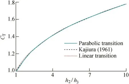
Fig.4.C T as function of h2/h3 for linear and parabolic transition cases,respectively,when L=10 m and ω=1.1922 s-1.

In this section,the numerical solution of Eq.(1),using a staggered conservative scheme,is presented.The scheme was described in detail in Pudjaprasetya and Magdalena(2014)and Magdalena et al.(2015).For the sake of concision,the scheme is described briefly here.We consider a computational domain Ω,consisting of a spatial domain ΩL= ［L0，L1］and a time domain ΩT= ［0，T］.The spatial domain ΩLis partitioned in a staggered way into several cells with a spatial step Δx.The time domain ΩTis discretized into finite time steps with a constant interval Δt.Momentum and mass conservation equations(Eq.(1))are discretized with cells centred atxiandxi+1/2,respectively.Furthermore,the water surface,η,and velocity,u,are defined at full-and half-grid points,respectively,as given in Fig.5.

The scheme leads to the numerical solutions of Eq.(1):

Fig.5.Discretization of staggered conservative scheme.

where superscripts and subscripts denote the time step and spatial grid point,respectively.As seen from Eq.(28),the water depth,h*,is required at half-grid points and is unknown.The value ofh*is approximated using a first-order upwind scheme and is chosen depending on the flow velocity as follows:

Note that on the right-hand side of the momentum equation(Eq.(1)),η is calculated attn+1,instead of attn,as this choice is required to maintain the stability of the scheme.Using Von Neumann stability analysis,the system is stable if|λ|＜ 1,where λ is the eigenvalue.The detailed derivation of the stability criteria for the numerical scheme can be found in Appendix A.Both the wave elevation and velocity are set to zero initially.As time passes,the wave is incident from the left,propagates over the sloping topography,and radiates through the right boundary.The initial and boundary conditions,respectively,are as follows:

whereAis the wave amplitude.

4.Results and discussion

To validate the numerical scheme,the numerical results were compared with the analytical solutions and the solution of Bautista et al.(2011).To study the influence of the sloping topography on the transmission and reflection of waves,the following parameter values were chosen.The constant depthh2was set as 10 m,the gravitational acceleration asg=9.81 m·s-2,the length of the sloping bottom asL=10 m,the time step as Δt=0.001 s,and the spatial step length as Δx=0.025 m.For the calculation,we used a monochromatic wave with a single crest.To calculate the amplitude of the reflected wave,the wave elevation at a certain point before the sloping bottom was observed,and then the maximum amplitude of the wave moving leftward,which was the reflected wave,was recorded.Comparisons of the transmission and reflection coefficients of those solutions are given in Figs.6 and 7,respectively.Fig.6 shows that the analytical and numerical solutions ofCTare in agreement.The solutions ofCTobtained in this study converge to that of Bautista et al.(2011)as ε→1,where ε=h3/h2.It can also be seen in Fig.7 that the solutions ofCRobtained in this study show the same trend,converging to that of Bautista et al.(2011)as ε→1.This is as expected as the WKB solution being valid for ε→1.The analytical and numerical solutions obtained in this study are in agreement with each other and extend the solution of Bautista et al.(2011)to the regime in which ε is not close to 1.

The differences between solutions,obtained by the analytical and numerical methods,for different values of ε are compared in Table 1,whereETandERare the absolute errors of the numerical results of the transmission and reflection coefficients,compared with their analytical results,respectively,withET=|CTn-CTa|andER=|CRn-CRa|.CTnandCTaare the transmission coefficients obtained by the numerical and analytical methods,respectively;andCRnandCRaare the reflection coefficients obtained by the numerical and analytical methods,respectively.

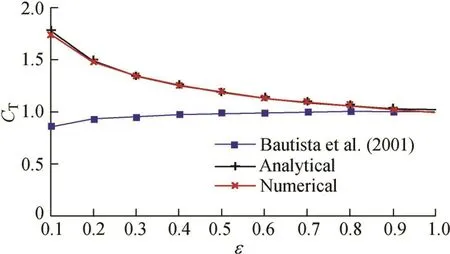
Fig.6.C T vs.ε.

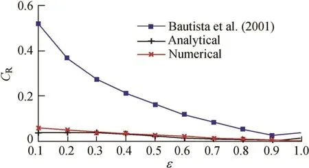
Fig.7.C R vs.ε.

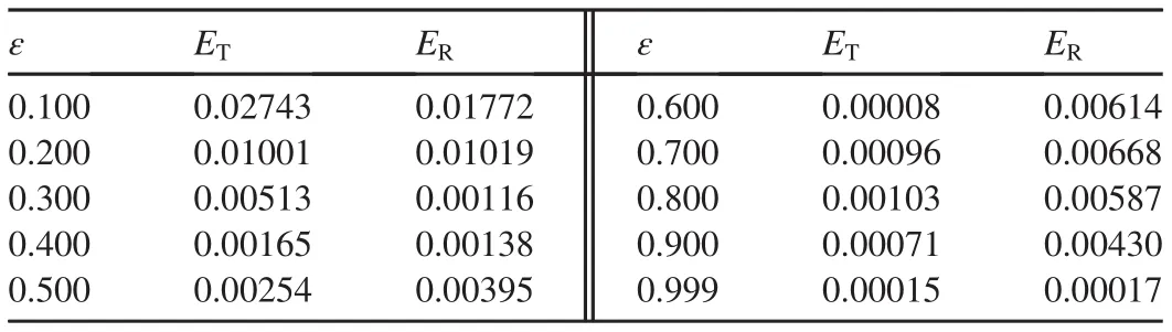
Table 1 Differences between analytical and numerical solutions of transmission and reflection coefficients.

It can be clearly seen from the table that the errors are very small.To investigate the accuracy of the numerical scheme proposed in this study,repeated simulations were conducted,with a fixed value of Δx=0.025 m and Δtranging from 0.000131 to 0.001831 s,to calculate the errorETjcorresponding to Δtjand the rate of convergence τtj=lg（ET（j+1）/ETj）/lg（Δtj+1/Δtj）.The results are shown in Table 2.Thein the range of 0-1,indicating that the order of accuracy in the time domain is one.

Next,to examine the accuracy of the numerical scheme in the spatial domain,repeated simulations were conducted,with Δt=0.001 s and Δxvarying between 0.010 m and 1.000 m,to calculateETjcorresponding to Δxjand the rate of convergence Table 3.The calculated value ofis in the range of 1.8-2.4,indicating that the order of accuracy in the spatial domain is two.We therefore concluded that the numerical scheme has an accuracy ofO（Δt，Δx2）(Pudjaprasetya and Magdalena,2014;Magdalena et al.,2015).

For a further test,results for a parabolic transition shelf were compared with those of Kajiura(1961).Thex-ordinate ran from-100 m to 0 m withx1=-60 m andx2=-40 m.The parametera=0.00625 m-1.The undisturbed water depths in deep and shallow areas were described byh2=andh3=,respectively.The wave propagated from the left with an amplitude ofai=0.5 m and a wave frequency of ω=5.9610 s-1.On the right side of the domain,an absorbing boundary condition was applied.The numerical result of the wave transmission coefficient was compared with those obtained by the analytical formula of Eq.(27)and from the literature,as shown in Tables 4 and 5,whereCTlis the wave transmission coefficient calculated from the formula derived by Kajiura(1961)and reproduced by Mei et al.(2005)using asymptotic expansions.The formula is valid only forx2-x1≫h2orh3,or when the water depth in the transition region with a sloping bottom strictly decreases in the shoreward direction.For example,in the case forx2=-50 m in Table 4,wherex2-x1=10 m is less thanh2=22.5 m andh3=15.625 m,the value ofCTlis far from the analytical and numerical results,demonstrating that Kajiura's formula is invalid.However,when all the parameters were chosen for the transition region with decreasing water depth under that condition,we could calculate the shoaling coefficient by inversion of the wave transmission coefficient given by Kajiura(1961)(Fig.4).

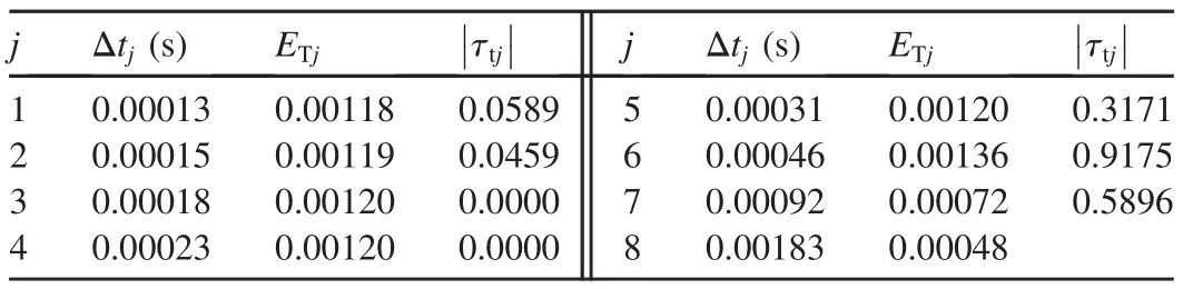
Table 2 Errors of numerical scheme and convergence rates for different time steps.

Table 3 Errors of numerical scheme and convergence rates for different spatial steps.

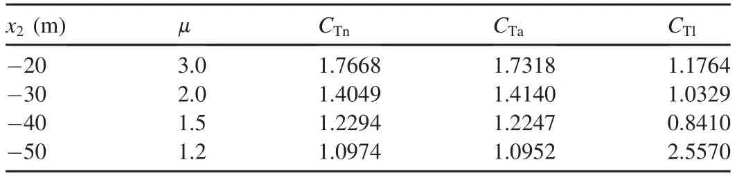
Table 4 Comparison of wave transmission coefficients for x1=-60 m,a=0.00625 m-1,and incident wave when a i=0.5 m and ω=5.9610 s-1.

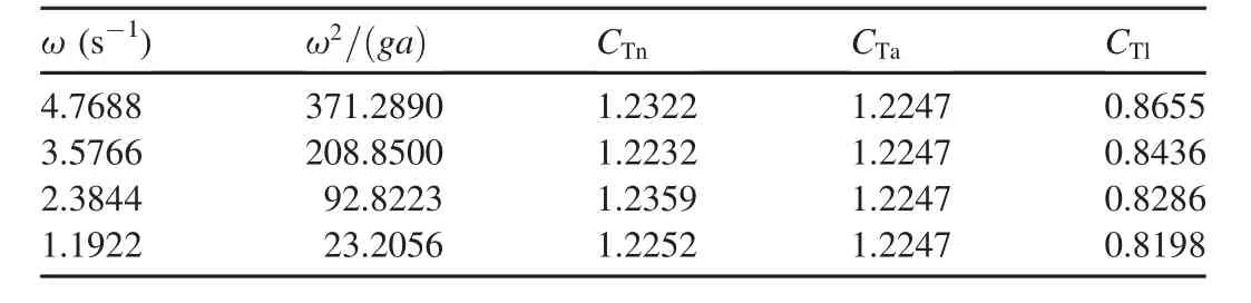
Table 5 Comparison of wave transmission coefficients forμ=1.5 and a=0.00625 m-1.

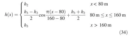
For a final test of the numerical scheme,a case in which the seabed transition was neither linear nor parabolic was chosen.The topography was determined as follows:

Finally,the numerical scheme was applied to simulation of the wave shoaling phenomena over a more complex bathymetry:a cross-sectional bathymetry of the coast of Aceh,in Sumatra,Indonesia,where the 2014 Boxing Day tsunami occurred.The cross-section was taken from (95.0278°E,3.2335°N)to(96.6583°E,3.6959°N)with Δx=0.4333 m.The wave propagating over the bathymetry along this crosssection is depicted in Fig.10.The incident wave with a 1-m wave height and a wave period of 17 min propagated to the shallow-water area.As the water depth decreased,wave

Monochromatic waves entered from the left with a wave amplitude of 0.5 m,and water depths were set ash2=22.5 m andh3=10 m.As time passed,the waves propagated to the shallow area and flowed through the right boundary.The computation was carried out in the spatial domain ranging from 0 to 250 m,with a spatial grid size of Δx=0.01 m.Fig.8 shows a comparison of the free surface elevation of the numerical solution in this study and the WKB solution described in Kristina et al.(2013).It is hard to distinguish between the two solutions for the free surface elevation in Fig.8.The WKB and numerical solutions are in close agreement.

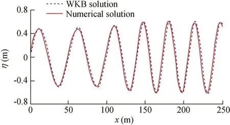
Fig.8.Free surface elevation of shoaling wave at t=50 s when h2=22.5 m and h3=10 m.

Fig.9.Wave transmission coefficients determined by numerical scheme and WKB method for ε in[0.1,0.9].

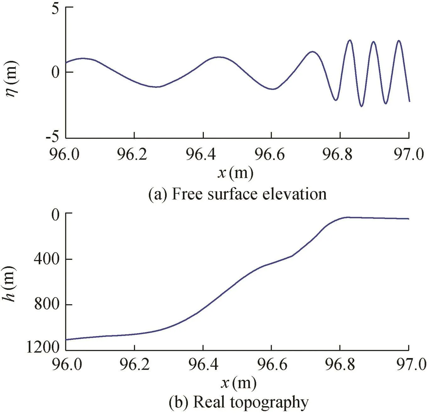
Fig.10.Transient wave propagating over cross-sectional bathymetry of coast of Aceh.

The wave transmission coefficient was calculated for different values of ε.Comparison of the calculated results with those of the WKB solution in Kristina et al.(2013)is shown in Fig.9.shoaling phenomena occurred,with the wavelength shortening and the amplitude increasing.For the domain shown,the water depth was 1047 m in the deep-water region and approximately 30 m in the shallow-water region.The wave height was 2.44 m in the shallow-water region,corresponding to a numerical solution of the wave transmission coefficient of 2.44.The analytical solution gave a transmission coefficient of 2.43 in this study,showing a reasonable agreement with the numerical solution.

5.Conclusions

In this paper,new analytical solutions for transient long waves shoaling over coastal shelves have been presented.Specifically,expressions for the surface elevation,horizontal velocity,and wave reflection and transmission coefficients have been derived for linear and parabolic transition shelves.Novel results from a numerical scheme have also been presented based on a staggered conservative formulation with upwind updating.The analytical and numerical solutions for several cases show agreement.The solutions obtained in this study have also been compared with previous results from WKB approximations,showing that this study provides a means of extending solutions beyond the normal WKB limits.The numerical scheme was applied to the case of tsunami propagation towards the coast of Aceh,Indonesia.Results obtained from the numerical scheme suggest that waves with a period of 17 min,close to values quoted by Stosius et al.(2010)for the Boxing Day tsunami,would experience amplification by a factor of 2.44 when traveling into the coastal waters where the depth was 30 m.This coincides with the scale of amplification proposed by Kowalik(2012),suggesting that the relatively simple approach proposed in this paper can provide solutions that are useful in practice,in either an operational or strategic context.

Appendix A.Stability analysis

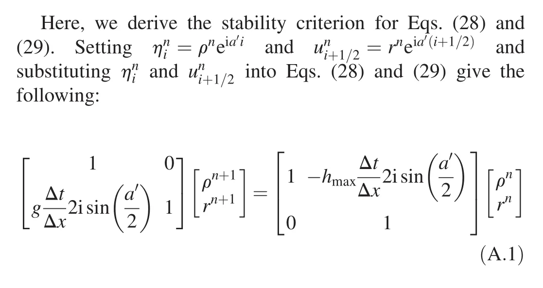
where ρ =eiωnΔt,with ωnbeing the angular frequency of η;a′=kΔx,withkbeing the wave number;r=eiωrΔt,with ωrbeing the angular frequency ofu;andhmaxis the maximum water depth.Eq.(A.1)can be rewritten as

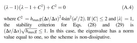
The eigenvalue λ of matrix B satisfies the following equation: