Assessment of future climate change impacts on hydrological behavior of Richmond River Catchment

Hshim Ism Jmeel Al-S fi*,Priynth Rnjn Srukklige

aDepartment of Civil Engineering,Curtin University,Perth 6102,Australia bDepartment of Irrigation and Drainage Techniques,Technical Institute of Shatrah,Southern Technical University,Dhi Qar,Iraq

Received 11 April 2016;accepted 5 May 2017 Available online 30 September 2017

Assessment of future climate change impacts on hydrological behavior of Richmond River Catchment

Hashim Isam Jameel Al-Sa fia,b,*,Priyantha Ranjan Sarukkaligea

aDepartment of Civil Engineering,Curtin University,Perth 6102,AustraliabDepartment of Irrigation and Drainage Techniques,Technical Institute of Shatrah,Southern Technical University,Dhi Qar,Iraq

Received 11 April 2016;accepted 5 May 2017 Available online 30 September 2017

This study evaluated the impacts of future climate change on the hydrological response of the Richmond River Catchment in New South Wales(NSW),Australia,using the conceptual rainfall-runoff modeling approach(the Hydrologiska Byrans Vattenbalansavdelning(HBV)model).Daily observations of rainfall,temperature,and stream flow and long-term monthly mean potential evapotranspiration from the meteorological and hydrological stations within the catchment for the period of 1972-2014 were used to run,calibrate,and validate the HBV model prior to the stream flow prediction.Future climate signals of rainfall and temperature were extracted from a multi-model ensemble of seven global climate models(GCMs)of the Coupled Model Intercomparison Project Phase 3(CMIP3)with three regional climate scenarios,A2,A1B,and B1.The calibrated HBV model was then forced with the ensemble mean of the downscaled daily rainfall and temperature to simulate daily future runoff at the catchment outlet for the early part(2016-2043),middle part(2044-2071),and late part(2072-2099)of the 21st century.All scenarios during the future periods present decreasing tendencies in the annual mean stream flow ranging between 1%and 24.3%as compared with the observed period.For the maximum and minimum flows,all scenarios during the early,middle,and late parts of the century revealed signi ficant declining tendencies in the annual mean maximum and minimum stream flows,ranging between 30%and 44.4%relative to the observed period.These findings can assist the water managers and the community of the Richmond River Catchment in managing the usage of future water resources in a more sustainable way.

©2017 Hohai University.Production and hosting by Elsevier B.V.This is an open access article under the CC BY-NC-ND license(http://creativecommons.org/licenses/by-nc-nd/4.0/).

Climate change impact;Hydrological modeling;HBV model;GCMs;Richmond River Catchment;Australia

1.Introduction

Future climate changes resulting from anthropogenic global warming constitute a growing problem for most of the world.Climate change can directly affect the availability of future water resources,mainly through changes in precipitation and temperature,and secondarily through changes in vegetation water use(Cheng et al.,2014).Several parts of the world aresuffering from water shortage as a result of climate change.Barron et al.(2011)reported that,since the mid-1970s,a noticeable climate shift in many parts of Australia has increased temperatures and reduced rainfall,resulting in a decline in the availability of local water resources.Numerous studies have con firmed this shift in the hydrological behavior across many local Australian catchments(Chiew et al.,1995,2009;Hennessy et al.,2007;CSIRO,2009;Bari et al.,2010;Silberstein et al.,2012;McFarlane et al.,2012;Islam et al.,2014;Al-Sa fiand Sarukkalige,2017).Since 1997,southeastern Australiahasexperienced asubstantialrainfall reduction with below-average long-term trends(1958-1998),which has badly impacted the current water resources in the region(Timbal and Jones,2008).According to the recent climate predictions,rainfall reduction trends are expected to continue in most parts of southeastern Australia as a result of global warming(Pittock,2003;CSIRO and BOM,2007).Consequently,the problems of below-average rainfall trends and the resulting stream flow decline require particular attention from the hydrological research community to establish a sustainable water resources management in the region and overcome the problem of water shortage.

The impacts of climate change on catchment hydrology can be estimated using hydrological modeling procedures.Climate change impact studies normally use the hydrological modeling approach to simulate the daily,monthly,and seasonal stream flow characteristics and predict the combined impact of climate change and other components on the hydrological status of local catchments(Chiew et al.,2009).Hydrological simulation at catchment scale usually requires the predictions of future climate conditions to simulate future stream flow at the catchment outlet.Future climate series of rainfall and temperature can be extracted from the analysis of global climate models(GCMs)at regional and global scales.According to Zorita and Storch(1999)and Solomon et al.(2007),GCMs represent a fair source for extracting the local and continental future climate signals.However,the resolution of climate series outputs resulting from GCMs is too coarse for direct use in catchment-scale hydrological modeling and needs to be downscaled before the simulation process(Fowler et al.,2007).Many hydrological studies have been conducted around the world to address the problem of climate change and its in fluence on future water demands(Kundzewicz et al.,2007;Bates et al.,2008;Praskievicz and Chang,2009;Whitehead et al.,2009;Driessen et al.,2010).Charles et al.(2010)pointed out that a plethora of hydrological impact studies with a diversity of GCMs and warming scenarios have provided warnings of an inevitable decline in future rainfall and runoff trends in many parts of Australia,and the currently available water resources will probably not meet the future demands for the continent.In short,the concern of diminished water accessibility in many Australian regions needs to be carefully addressed in order to achieve consistent water management and to meet the future water demands in these areas.

The main objective of the present work was to assess future climate change impacts on the hydrological behavior of the Richmond River Catchment in New South Wales(NSW),Australia.The study involved the application of a conceptual lumped-parameters Hydrologiska Byrans Vattenbalansavdelning(HBV)model to perform the hydrological modeling.Global-scale future climate series(monthly mean outputs)were obtained from a multi-model ensemble of seven GCMs of the Coupled Model Intercomparison Project Phase 3(CMIP3)for three climate scenarios:A2,B1,and A1B.The data came from the Intragovernmental Panel on Climate Change Fourth Assessment Report(IPCC-AR4)of the World Climate Research Programme(WCRP).According to the Special Report on Emission Scenarios(IPCC,2000),the A2 scenario represents a very heterogeneous world with continuous population growth,slow economic and technological development,and the average CO2emission reaching 850 ppm by the end of this century.The B1 scenario is a convergent world with a global population that peaks by the middle of the 21st century and decreases afterwards with rapid economic and technological development.For the B1 scenario,the average concentration of CO2emission first increases at the same rate as it does in the A2 scenario,and then decreases near the mid-century,reaching 550 ppm (IPCC,2000).Meanwhile,the A1B scenario represents a balanced status across all energy sources.The Long Ashton Research Station Weather Generator Version 5.5(LARS-WG 5.5)was utilized in this study to extract the local-scale daily future rainfall and temperature from each of the seven GCMs'outputs.The ensemble mean of the downscaled seven GCMs was then derived and used as input data to force the HBV rainfall-runoff model to simulate the future daily stream flow at the Casino Gauging Station on the Richmond River.The outcomes of this research can deliver effective water management policies in the study area and help to overcome the problem of low water accessibility in the future.

2.Catchment description

The Richmond River Catchment,with an approximate area of 7000 km2,is located in the distant northern part of NSW,Australia.It extends from the Border Ranges in the north to the Richmond Ranges in the west and south,with variable elevation,ranging from a few meters above sea level near the coastal floodplain to more than 1000 m above sea level near the Border Ranges.The area includes World Heritage sites and diverse geography,including rainforest,agricultural lands,and coastal estuaries.The catchment also comprises popular tourist places such as Ballina and supports a continuously growing population attracted by the region's coastal lifestyle.Furthermore,it holds extensive agricultural lands and wetlands,which consume high quantities of water.Therefore,the impact of future climate change on the local water resources in the catchment is highly signi ficant to designing ef ficient and sustainable water management strategies in the area.In the present work,the area upstream the Casino Gauging Station was taken into consideration(Fig.1),as it holds a continuous record of hydrometeorological data for a period of 43 years(1972-2014).It stretches between the latitudes of 28.00°S to 29.30°S and longitudes of 152.15°E to 153.15°E and encompasses an approximate drainage area of 1790 km2.The catchment has Mediterranean climatic conditions with a relatively warm dry summer,approximately ranging between 27°C and 30°C,and a moderate winter ranging between 19°C and 20°C(CSIRO and BOM,2007).The period between November and April includes the peak rainfall,which varies between 1350 and 1650 mm/year in the catchment's coastal areas,whereas the interior areas receive the lowest amount of precipitation,under 800mm/year at Armidale(CSIRO and BOM,2007).

3.Datasets

3.1.Observed climate data

A daily-scale continuous hydro-meteorological record for a period of 43 years(1972-2014)was available for the study area.Daily observed mean values of rainfall,temperature,and stream flow,and thelong-term monthly mean potential evapotranspiration were obtained from seven meteorological stations and one hydrological station and included in the hydrological modeling(Table 1).The locations of the hydrometeorological stations are illustrated in Fig.1.The recorded data were provided by the Australian Bureau of Meteorology(BOM),and the quality of data was checked carefully.The average areal precipitation over the catchment was obtained through the Thiessen polygon method.

3.2.Future climate data

Data from regional climate scenarios can be used to force hydrological models(for instance the HBV model)to simulate the climate change impact on catchment hydrology.Fu et al.(2007)explained that the GCMs'outputs always involve uncertainties that result from using different climate scenarios.Therefore,an ensemble analysis that combines multiple GCM projections and quanti fication of the probability of future climatic conditions is usually used to create more consistent regional climate scenarios.In the present work,the globalscale future rainfall and temperature(monthly mean outputs)were extracted from a multi-model ensemble of seven GCMs of the CMIP3(Table 2)for three climate scenarios,A2,A1B,and B1,from the IPCC-AR4.These models effectively reproduce the observed historical mean annual rainfall and the daily rainfall distribution across southeastern Australia based on a combined score rank provided by Vaze et al.(2011).

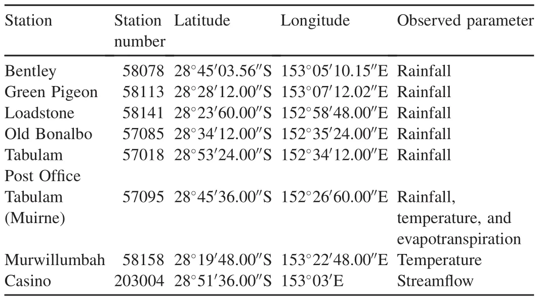
Table 1 Locations of hydrological and meteorological stations.

Next,the global-scale outputs were transferred(downscaled)into daily local-scale climate projections suitable for regional impact assessment studies using the LARS-WG 5.5 stochastic weather generator(a detailed description is provided in Sections 5.2 and 6.1).The ensemble mean of the downscaled seven GCMs was then derived and adopted.The future data spans the current century into three future periods,the near future(2016-2043),the middle part of the 21st century(2044-2071),and late part(2072-2099)of the 21st century.Depending on the downscaled daily mean temperature,the modi fied Blaney-Criddle method(Eq.(1))(Doorenbos and Pruitt,1977)was employed to obtain the potential evapotranspiration across the catchment for the future periods.Palutikof et al.(1994)explained that this method computes the potential evapotranspiration by utilizing the daily mean temperature （Tmean）and daily mean proportion of annual daylight hours(D)on the condition that Tmeanis not less than-8°C.As the future daily mean temperatures across the catchment are anticipated to be higher than 0°C,this method provides easy access to future potential evapotranspiration across the catchment for the future periods.

where PEis the monthly average crop evapotranspiration(mm/d),and C is a correction factor that depends on sunshine hours,minimum relative humidity,and daytime wind speed.

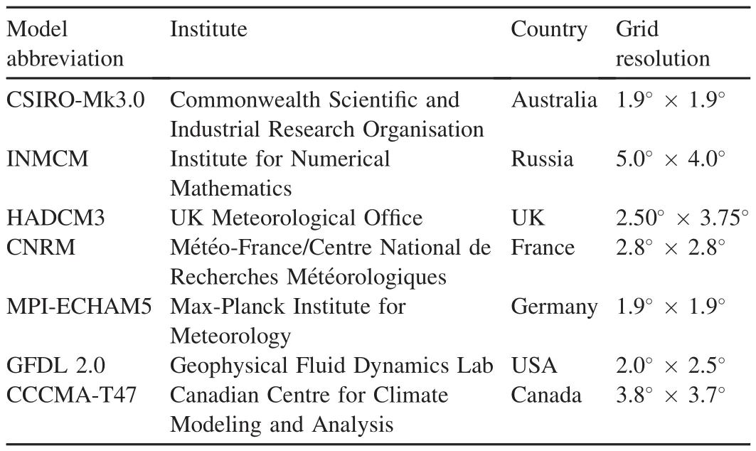
Table 2 Seven GCMs of CMIP3 included in present study.

4.Hydrological modeling

The Swedish conceptual lumped-parameter(HBV model version7.3)(SMHI,2012)was used in this study to perform the hydrological modeling.The HBV model can be classi fied as a semi-distributed rainfall-runoff model of catchment hydrology.It depends on the daily rainfall,air temperature,and long-term monthly mean potential evapotranspiration as input data to simulate the daily stream flow at a basin outlet(Bergstrom,1995;SMHI,2012).Lindstrom et al.(1997)reported that the HBV model had proven its high level of performance in many regions around the world with a diversity of climatic conditions,where different versions of the model have been successfully used to perform the hydrological modeling.SMHI(2012)explained that the HBV model includes four key components:a precipitation routine,a soil moisture routine,river routing,and a response routine.Three storage reservoirs are usedbytheHBVmodeltode fine thewaterbalancemechanism,including a storage for soil moisture,and upper and lower zone storages(SM,UZ,and LZ,respectively)(SMHI,2012).Therefore,Eq.(2)can provide a general description of the water balance equation(Liden and Harlin,2000).More information about the HBV model can be found in SMHI(2012).

where P,E,L,ΔS,and Q refer to the precipitation,evapotranspiration,losses to groundwater systems or nearby catchments,water storage variation,and the excess runoff from the basin,respectively.

The Richmond River Catchment can be considered a nonsnow area.Therefore,the precipitation routine in this study was represented by rainfall only.The soil moisture routine can be represented by three parameters,namely, field capacity（Fc）,the parameter β,and the limits of potential evaporation（Lp）,which provides an estimation of the water content in the catchment's soil(Abebe et al.,2010).Fcrefers to the extreme soil storage capacity of the catchment,β governs the relative participation of rainfall in the volume of runoff for a speci fied soil moisture de ficit,and Lpgoverns the format of the potential evapotranspiration curve.The surplus water of the soil moisture routine is transformed through the response routine for release into catchment storage through two connected reservoirs(UZ and LZ).These reservoirs are connected by a filtration rate（PERC）in which water percolates from the UZ to the LZ at a constant proportion(Abebe et al.,2010).The channel flow hydraulics(runoff)can be described by the transformation function parameter（MAXBAZ）,which calculates the collected out flow from the catchment.

5.Methodology

5.1.Model calibration,validation,and parameter estimation

A daily observed stream flow record with a variety of hydrological regimes is required to calibrate and validate the HBV model with greater accuracy.For the Richmond River Catchment,daily stream flow observations at the Casino Gauging Station on the Richmond River were available for 43 years(1972-2014).According to Vaze et al.(2010),the recent stream flow records from the southeastern Australian catchments can be used effectively to calibrate process-based models to represent the current prolonged drought across the region.They can also be used successfully to predict the future climate change impact on the local catchments where the vast majority of climate models predict a drier future across this region.The HBV model was first run for an initial state of one year(1972-1973)to initialize the system.Then,the model was calibrated and validated manually against the daily observed stream flow data for the periods of 1973-2000 and 2001-2014,respectively.Driessen et al.(2010)suggested that long calibration periods of hydrological models could be useful for the simulation of large datasets of future scenarios.Hence,a calibration period twice as long as the validation period was used in the present work.

Nine parameters were included in the calibration process.The resulting set of the optimal parameters and the order in which they were optimized is presented in Table 3.SMHI(2012)explained that the method of evaluating the results during the calibration process is highly signi ficant.Therefore,the modeling performance was assessed using three criteria of ef ficiency,Nash-Sutcliffe ef ficiency (NSE) (Nash and Sutcliffe,1970),the relative volume error （VE）,and the coef ficient of determination(r2)(Eqs.(3)through(5)).According to SMHI(2012),for high-quality input data,the NSE criteria ranged between 0.8 and 0.95.Reasonable modeling results were achieved during the calibration and validation processes(Table 4),which indicate that the model can be used effectively for climate change impact assessment purposes.Fig.2 illustrates a comparison between the observed and simulated stream flows at the Casino Gauging Station for the calibration and validation periods.The hydrographs appear only at speci fied intervals,November 1998 to July 2000 and September 2010 to September 2011,to enable a clear comparison between the observed and simulated hydrographs,especially in low- flow periods.Fig.2 shows that the calculated and observed hydrographs are in good agreement for the high and medium flows,except for some periods of low- flowsimulations.This can be attributed to the fact that the conceptual structure of the HBV model is relatively simple,with only a single groundwater storage value responsible for the runoff generation.

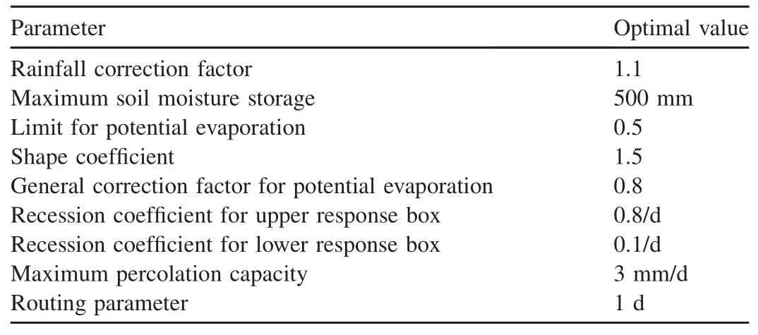
Table 3 HBV model parameters and their optimal values for calibration and validation periods.

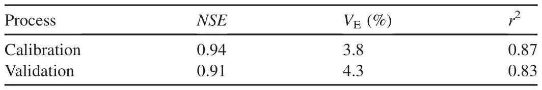
Table 4 HBV model performance during calibration and validation periods.

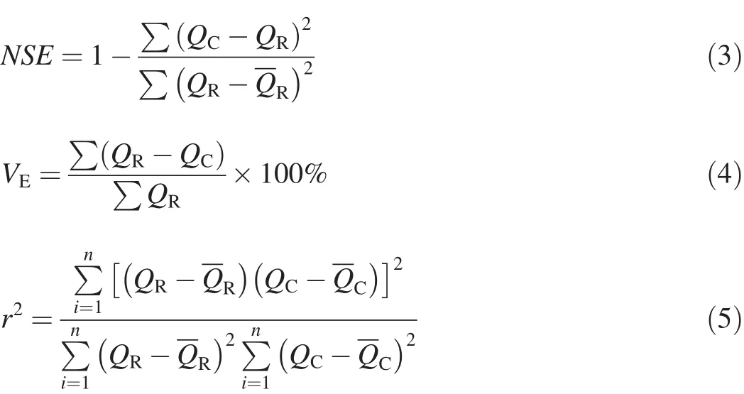
where QCand QRare the computed and observed stream flows,andare the mean observed and calculated stream flows over the calibration period,respectively.

5.2.Data downscaling

Despite the improved general resolutions of the CMIP3,its spatial and temporal resolutions are still too coarse for direct application to local-scale impact assessment studies.Therefore,the GCM outputs need to be downscaled to a finer scale to be used effectively as inputs to the rainfall-runoff models.Many downscaling techniques are globally available to extract the regional-scale of GCM outputs,including statistical downscaling(Charles et al.,2004;Fowler et al.,2007),dynamic downscaling(Gordon and O'Farrell,1997;Nunez and McGregor,2007),and weather generators(Semenov and Barrow,1997).In this study,we utilized LARS-WG 5.5,a highly popular stochastic weather generator(Semenov and Stratonovitch,2010),to extract the local-scale rainfall and temperature from each GCM of the CMIP3 ensemble for the early,middle,and late periods of the 21st century.LARS-WG 5.5 is a statistical downscaling model(Wilks and Wilby,1999)used to generate local-scale daily weather data required for climate change impact studies.Semenov and Barrow(1997)simulated the magnitude and periodic sequence of the main climate features ef ficiently with the LARS-WG model.This downscaling technique provides a cross-validation for the generated data,which has signi ficantly improved the simulation of extreme weather events(Semenov and Stratonovitch,2010).Accordingly,it has been successfully applied in many local-impact assessment studies on diverse climates and has proven its applicability as well as its high performance,where bias corrections or any other adjustments are not required(Semenov and Stratonovitch,2010;Gunawardhana et al.,2015).

The weather data generation process using the LARS-WG model is as follows(Semenov and Barrow,2002):

(1)Model calibration:The model analyzes the daily observed weather parameters (rainfall,minimum and maximum temperatures,and solar radiation)of a speci fied location during a baseline period to determine their statistical characteristics.Then,it creates a set of calibrated probability distribution parameters for that site to be stored in two parameter files.

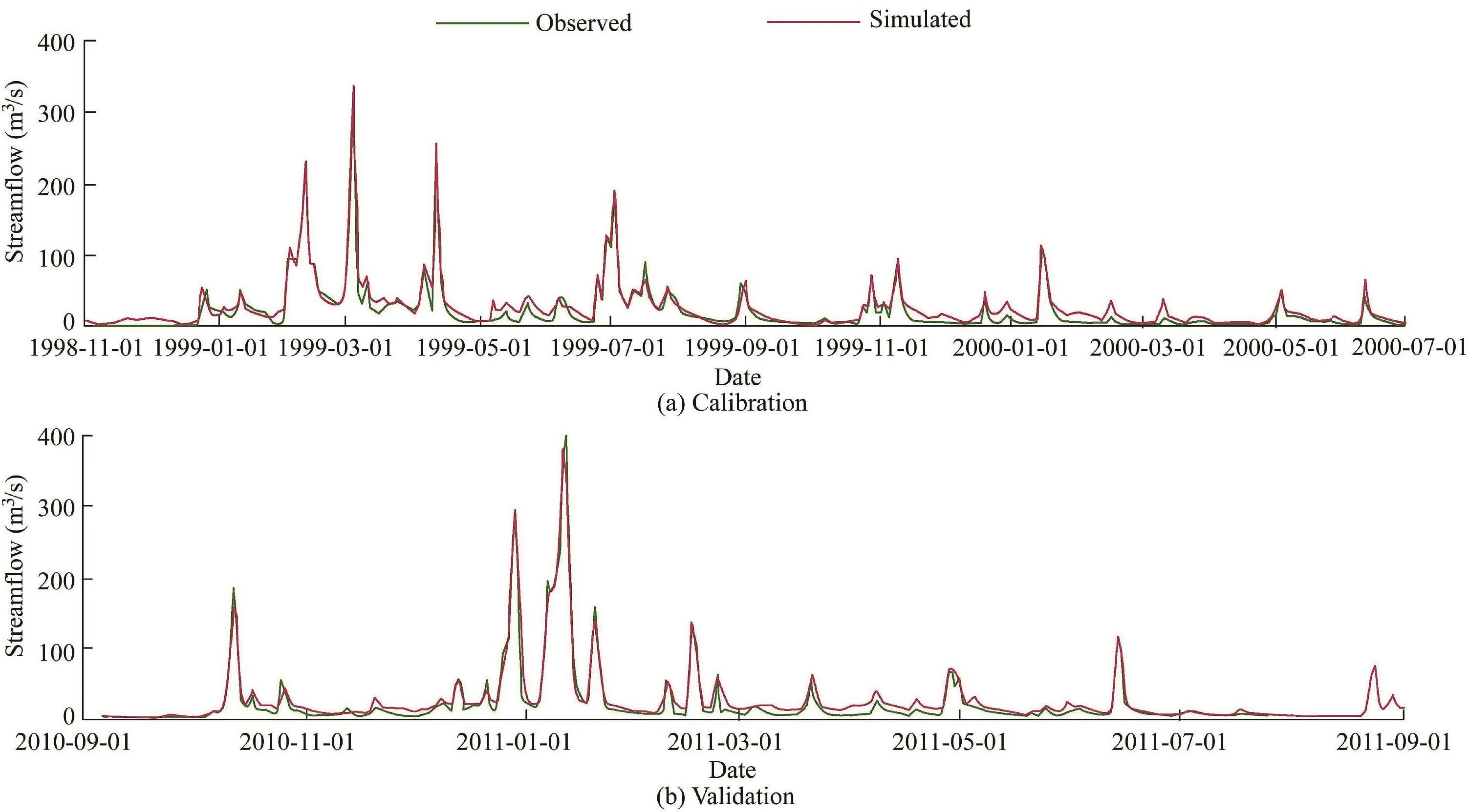
Fig.2.Calibration and validation results at Casino Gauging Station on Richmond River.

(2)Model validation:The created parameter files are used to generate synthetic climate data with the same statistical characteristics as the original observed data.The validity of the model is examined by comparing the statistical features of the observed and synthetic data to evaluate the LARS-WG model's suitability for simulating future weather data for that site.

(3)Climate scenario generation:By perturbing the calibrated parameters of the selected site with the monthly-scale climate predictions derived from global or regional climate models,a daily climate scenario for that site can be generated.

The model utilizes a semi-empirical probability distribution(SED)to estimate probability distributions of dry and wet series of daily climate parameters(Semenov and Barrow,2002).SED is de fined as a separate histogram that has a constant number of intervals of adjustable lengths.The wet days are de fined as the days with precipitation.The LARSWG 5.5 model uses 23 intervals to describe the shape of the SED compared to the ten intervals of the earlier versions(Semenov and Stratonovitch,2010).This allows various distributions of weather statistics(rainfall and temperature)to be simulated more accurately.The simulation of daily temperature statistics(minimum and maximum)is governed by the status of the day whether it is wet or dry.A relatively long record of daily observed weather(minimum of 20 years)is required to obtain robustly calibrated weather parameters,which are used later to produce the synthetic future data(Semenov and Barrow,1997).In this study,40 years(1972-2011)of observed daily rainfall,as well as minimum and maximum temperatures from seven weather stations(sites)were utilized as a baseline period to create the calibrated weather parameters.These parameters were then adjusted by the Delta-changes for the derivation of future climate scenarios using each of the seven GCMs that covered the proposed site to generate catchment-scale future daily time series of rainfall and temperature at that site.Finally,the ensemble mean of the local-scale climate outputs was used to force the HBV model to simulate the future daily stream flow at the Casino Gauging Station on the Richmond River.

Using the daily recorded site weather parameters in line with the monthly-scale climate outputs resulting from each of the seven GCMs,LARS-WG 5.5 can produce daily climate series for the site that are statistically similar to the CMIP3 climate projections.By treating each GCM prediction from the CMIP3 ensemble as an equally possible evolution of climate,we can explore the uncertainty in the impact assessment resulting from the uncertainty in climate projections.

6.Results and discussion

6.1.Performance of LARS-WG 5.5

The ability of LARS-WG 5.5 to capture the observed climate data should be checked before generation of the future climate series of rainfall and temperature required for climate impact assessment. As mentioned earlier, 40 years(1972-2011)of observed daily precipitation as well as minimum and maximum temperatures were used to calibrate and validate LARSE-WG 5.5.The modeling performance was assessed by relating the probability distributions of the generated(synthetic)climate data with those resulting from the observations.For the rainfall time series,two characteristics were used:monthly mean rainfall and standard deviation(Fig.3),while for the temperature time series,the minimum and maximum monthly mean statistics were taken into account(Fig.4).Figs.3 and 4 clearly show that the simulated rainfall and temperature statistics strongly agree with those of the observed data.

The Kolmogorov-Smirnov(K-S)test was performed to compare the seasonal probability distributions for the lengths of the wet/dry periods(Table 5).The K-S test was also used to assess the equality of the daily distributions of rainfall as well as minimum and maximum temperatures calculated from the observed and simulated data series(Tables 6 and 7).The test computes a p-value,which gives an indication of the possibility that the observed and generated datasets may have come from the same distribution.A very small p-value(corresponding to a high K-S value)indicates that the synthetic data belong to a distribution different from that of the observed climatic data,and therefore it should be rejected,while a large p-value means that the differences between the observed and generated climate statistics for the variable in consideration are too small and therefore it is accepted.Semenov and Barrow(2002)recommended that a p-value of 0.01 be used as the acceptable signi ficance limit of the model results.

Fig.3.Comparison between observed and generated rainfall time series.

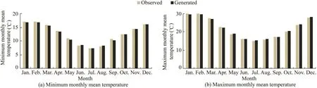
Fig.4.Comparison between observed and generated temperature time series.

Table 5 demonstrates the proper performance of the LARSWG model in simulating the seasonal distributions of the wet and dry periods.In addition,the daily distributions of rainfall as well as minimum and maximum temperatures(Tables 6 and 7)verify the excellent modeling performance.It can be seen that all p-values in Tables 5 through 7 are greater than 0.01(i.e.,a 99%con fidence level)and the results of the assessment columns ranged between a good and perfect fit.The seasonal distributions of the wet/dry periods in line with the daily rainfall and minimum and maximum temperature distributions are vital when the model results are used in impact assessment studies(Osman et al.,2014).As these properties werecorrectly fitted,the calibrated parameters derived from the observed weather data can be incorporated properly with the future climate scenarios to generate daily rainfall and temperature time series for climate impact assessment in the Richmond River Catchment.

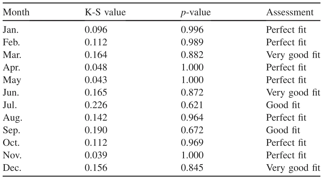
Table 6 K-S test results for daily rainfall distributions in each month.

Table 7 K-S test results for daily minimum and maximum temperature distributions in each month.

6.2.Future climate projections

Table 8 provides an overview of the annual mean precipitation （P′）,temperature （T）,and PEfor the future periods across the Richmond River Catchment and their comparison with the observed ones.In the table,all values of future climate variables represent the ensemble mean of the seven GCMs.During the observed period of 1972-2014,P′was 1209 mm/year,T was 17.5°C,and PEwas 1553 mm/year.Almost all GCMs predict reduction tendencies in rainfall and an increase in temperature and potential evapotranspiration under all future scenarios,except for the early century,which includes a slight increase in rainfall amounts.For the nearfuture part of the 21st century,all GCMs of the multi-model ensemble predict a small increase in the mean annual rainfall of 3%,0.8%,and 2.3%for scenarios A2,A1B,and B1 respectively,compared to the observations.By mid-century,the mean annual rainfall shows a slight decrease of 2%,2.8%,and 4%for the A2,A1B,and B1 climate scenarios,

Period Scenario P′(mm/year) Change in P′(%) T(°C) Change in T(°C) PE(mm/year) Change in PE(%)respectively,as compared with the recorded period,while by late century the average decline in mean annual rainfall relative to the observed climate is predicted to be 4.7%,10%,and 6.5%for the same scenarios.The historical analysis of observed annual rainfall across southeastern Australia shows decreasing trends over the time.Since 1997 the average annual rainfall has declined by more than 25%below the long-term averagetrend (1958-1998)(Trewin andJones,2004).Therefore,this pattern of change across the study area,which started in 1997,is expected to continue during the middle and late periods of the current century.

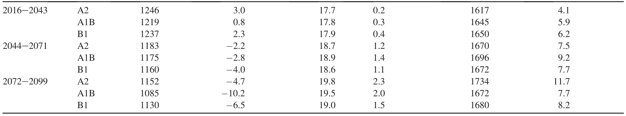
Table 8 An overview of mean annual precipitation,temperature,and potential evapotranspiration across Richmond River Catchment(from seven meteorological stations)for projected periods,and their comparison with those of observed period.

On the other hand,annual mean temperature values show positive trends for all climate scenarios of the future periods compared to the observations.This expected rise in temperature will lead to an increase in the mean annual potential evapotranspiration by approximately 6.2%,9.2%,and 11.7%,respectively,by the early,middle,and late periods of the century across the study area.A possible explanation for this increment in future potential evapotranspiration is the use of the modi fied Blaney-Criddle method,which is directly related to the daily mean temperature to derive PE.As the daily mean temperature is expected to rise in the future,additional energy is available for driving soil water and intercepted water for evaporation or transpiration.Consequently,the combined impact of rainfall reduction and the potential evapotranspiration increase by the middle and late periods of the century could adversely impact the future stream flow across the catchment.

6.3.Future stream flow simulation

The calibrated HBV model was forced with the ensemble mean of the downscaled future climate signals to simulate the future daily stream flow at the Casino Gauging Station for the early,middle,and late periods of the 21st century for the A2,A1B,and B1 climate scenarios.A time interval of 28 years per scenario was selected for the future periods to ensure that the simulation periods were equal to the calibration period(1973-2000).Vaze et al.(2010)explained that the rainfallrunoff models calibrated over a period of more than 20 years could be used ef ficiently in the impact assessment studies under the condition that the future mean annual rainfall is neither more than 15%drier nor 20%wetter than in the calibration period.As the projected mean annual rainfall across the Richmond River Catchment is within that range,in contrast to the observed annual mean rainfall over the 28-year calibration period(Table 8),the calibrated HBV model can be used competently to predict the impact of climate change on catchment hydrology.As stated by Driessen et al.(2010),to consider different model simulations,three stream flow statistics at the Casino Gauging Station were created,including annual mean stream flow （Qmean）,annual mean maximum stream flow （Qmax）,and annual mean minimum stream flow（Qmin）.These statistics were derived from three different datasets,including observed stream flow,stream flow resulting from forcing the HBV model with the recorded climate(from the seven meteorological stations),and stream flow derived from forcing the calibrated HBV model by the three future climate scenarios,A2,A1B,and B1(Table 9).During the observed period(1972-2014),Qmeanwas 19.9 m3/s,Qmaxwas 589.76 m3/s,and Qminwas 0.63 m3/s.Stream flow statistics resulting from forcing the HBV model with the observed climate data were as follows:Qmeanwas 21.02 m3/s,Qmaxwas 570.19 m3/s,and Qminwas 0.52 m3/s.The same set of model parameters(Table 3)was used to simulate the future streamfl ow across the catchment(Vaze et al.,2010).Fig.5 illustrates a comparison between the observed stream flow and the stream flow resulting from forcing the HBV model with the observed climate data.Fig.6 shows the simulation results of future stream flow at the Casino Gauging Station for the three future climate scenarios.

Table 9 and Fig.6 clearly show the response of the Richmond River Catchment to the anticipated climate change impact through the decline in all future stream flow statistics measured at the Casino Gauging Station.Despite the slight increase in the annual mean rainfall during the near future,all annual stream flow statistics revealed small reduction tendencies for all scenarios.The annual mean stream flow is projected to decrease slightly by 2.5%,5.8%,and 1%for the A2,A1B,and B1 scenarios,respectively,compared to the observed stream flow,while the minimum and maximum stream flow statistics are also projected to decline within arange of 30%-44.4%for the same scenarios relative to the observations.This is most likely due to the relative increase in potential evapotranspiration across the catchment.Another possible explanation is that the small rainfall increment has been used by the model to bring the soil of the catchment into its maximum storage capacity （FC）.Therefore,the HBV model does not include this increase in the runoff calculations.By mid-century,the annual mean stream flow is projected to decline by 4.6%,8.3%,and 13.5%for the A2,A1B,and B1 climate scenarios,respectively,compared to the recorded stream flow.The minimum and maximum stream flows are also expected to decline within a range of

30.3%-39.7%for the same scenarios relative to the observations.Similarly,by the end of the 21st century,all stream flow statistics are expected to decrease within a range of 18.3%-24.3%for the annual mean stream flow and 35.43%-44.4%for the annual mean minimum and maximum flows,compared to the recorded stream flow.

Table 9Future stream flow statistics(annual mean,annual mean maximum,and annual mean minimum stream flows)for three climate scenarios and their comparison with those of observed period.

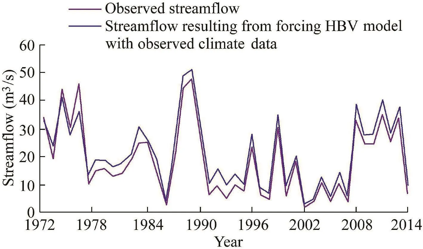
Fig.5.Comparison between observed annual mean stream flow at Casino Gauging Station and simulated stream flow resulting from forcing HBV model with observed climate data.

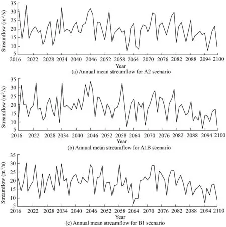
Fig.6.Future annual mean stream flows at Casino Gauging Station for three climate scenarios(future stream flow is ensemble mean of seven GCMs).

Based on these results,the HBV conceptual model was successfully used to predict the impact of future climate changes on the hydrological behavior of the Richmond River Catchment.The outcomes of this study align with previous studies that have been implemented in other basins of southeastern Australia and displayed an apparent decline in future stream flow.For instance,Chiew et al.(2009)and Vaze and Teng(2011)showed that the future stream flow across many local catchments in southeastern Australia is projected to decline within a range of 0-20%by 2030.They used the IPCC-AR4 climate scenarios informed by 15 GCMs under median emission projections(the A1B climate scenario)to force the SIMHYD(a simpli fied version of the daily conceptual rainfall-runoff model HYDROLOG)and Sacramento conceptual rainfall-runoff models to simulate the future stream flow across the catchments.Teng et al.(2012a)also used the climate projections informed by 15 GCMs of the CMIP3 to force five conceptual rainfall-runoff models to simulate the future stream flow across southeastern Australia.They found that the majority of the modeling results indicate a larger reduction in future runoff across the study area by the middle of the 21st century.Another study by Teng et al.(2012b)also revealed a clear reduction in the future runoff across the southeast and far southwest of the Australian continent.In addition,the more recent studies implemented by the researchers of the CSIRO and BOM(2015)have con firmed that the rainfall-runoff trends in most parts of southeastern Australia are projected to decline through the middle and late periods of the 21st century.

7.Conclusions

Future climate change impactson the hydrological behavior of the Richmond River Catchment during the 21st century were investigated for three future climate scenarios:A2,A1B,and B1.The following conclusions from this study can be drawn:

(1)Overall modeling results of the seven GCMs show that rainfall is projected to increase slightly during the near-future and decrease during the middle and late periods of the century for all climate scenarios compared to the observations from 1972 to 2014.Potential evapotranspiration is also projected to increase for all scenarios during the future periods due to the relative increase in annual mean temperature relative to the observed period.

(2)Comparison of the observed and future simulated stream flows across the study area shows that the hydrological status of the catchment is likely to change signi ficantly.The annual mean stream flow measured at the Casino Gauging Station is projected to decline for all scenarios during the future periods.The average annual maximum and minimum stream flows are also expected to decrease signi ficantly for all scenarios of the future periods.

(3)This study highlights the similar outcomes of other previous studies that have been implemented in other southeastern Australian catchments and revealed noticeable rainfallrunoff reduction trends.

(4)The projected annual stream flow reduction could signi ficantly impact the currently available surface water resources in the area and in fluence the environmental and aquatic life of the Richmond River system.

(5)The potential impacts of future climate changes in line with the continuous economic and population growth in the catchment will impose additional burdens on the currently available water resources,which will probably not meet the future demands.Therefore,long-term development plans in the area should take into account the potential effect of climate change in order to design sustainable and ef ficient water management strategies to overcome the problem of water scarcity.

(6)The outcomes of the present study could assist the authorities and the community of the Richmond River Catchment in managing the usage of future water resources in the catchment,taking into consideration the low- flow situation.They could also be signi ficant to preserving the extensive wetland complexes in the lower Richmond River,such as Tuckean Swamp on the Richmond floodplain and Ballina Nature Reserve,which protect wide areas of mangroves and saltmarsh communities from the risk of streamfl ow reduction.

Acknowledgements

The authors would like to acknowledge the financial support of the Higher Committee for Educational Development in Iraq(HCED Iraq)for sponsorship of this study.

Abebe,N.A.,Ogden,F.L.,Pradhan,N.R.,2010.Sensitivity and uncertainty analysis of the conceptual HBV rainfall-runoff model:Implications for parameter estimation.J.Hydrol.389(3-4),301-310.https://doi.org/10.1016/j.jhydrol.2010.06.007.

Al-Sa fi,H.I.J.,Sarukkalige,P.R.,2017.Potential climate change impacts on the hydrological system of the Harvey River Catchment.Int.J.Environ.Chem.Ecol.Geol.Geophys.Eng.11(4),296-306.

Bari,M.A.,Amirthanathan,G.E.,Timbal,B.,2010.Climate change and long term water availability in Western Australia:An experimental projection.In:Proceedings of International Congress on Environmental Modelling and Software.Melbourne,pp.1-9.

Barron,O.V.,Crosbie,R.S.,Charles,S.P.,Dawes,W.R.,Ali,R.,Evans,W.R.,Cresswell,R.,Pollock,D.,Hodgson,G.,Currie,D.,et al.,2011.Climate change impact on groundwater resources in Australia:Summary report.Commonwealth Scienti fic and Industrial Research Organization(CSIRO),Canberra.

Bates,B.,Kundzewicz,Z.W.,Wu,S.H.,Palutikof,J.,2008.Climate Change and Water.Intergovernmental Panel on Climate Change(IPCC),Geneva.

Bergstrom,S.,1995.The HBV-model.In:Singh,V.P.(Ed.),Computer Models for WatershedHydrology.WaterResourcesPublications,Colorado,pp.443-476.

Charles,S.,Silberstein,R.,Teng,J.,Fu,G.B.,Hodgson,G.,Gabrovsek,C.,Crute,J.,Chiew,F.,Smith,I.,Kirono,D.,et al.,2010.Climate analyses for south-west western Australia:A report to the Australian Government from the CSIRO South-West Western Australia Sustainable Yields Project.Commonwealth Scienti fic and Industrial Research Organization(CSIRO),Canberra.

Charles,S.P.,Bates,B.C.,Smith,I.N.,Hughes,J.P.,2004.Statisticaldownscalingof daily precipitation from observed and modelled atmospheric fields.Hydrol.Process.18(8),1373-1394.https://doi.org/10.1002/hyp.1418.

Cheng,L.,Zhang,L.,Wang,Y.P.,Yu,Q.,Eamus,D.,O'Grady,A.,2014.Impacts of elevated CO2,climate change and their interactions on water budgets in four different catchments in Australia.J.Hydrol.519(B),1350-1361.https://doi.org/10.1016/j.jhydrol.2014.09.020.

Chiew,F.H.S.,Whetton,P.H.,McMahon,T.A.,Pittock,A.B.,1995.Simulation of the impacts of climate change on runoff and soil moisture in Australian catchments.J.Hydrol.167(1-4),121-147.https://doi.org/10.1016/0022-1694(94)02649-V.

Chiew,F.H.S.,Teng,J.,Vaze,J.,Post,D.A.,Perraud,J.M.,Kirono,D.G.C.,Viney,N.R.,2009.Estimating climate change impact on runoff across southeast Australia:Method,results,and implications of the modelling method.WaterResour.Res.45(10),W10414.https://doi.org/10.1029/2008WR007338.

Commonwealth Scienti fic and Industrial Research Organization(CSIRO)and Bureau of Meteorology(BOM),2007.Climate Change in Australia.Melbourne.

Commonwealth Scienti fic and Industrial Research Organization(CSIRO),2009.Surface Water Yields in South-west Western Australia:A Report to the Australian Government from the CSIRO South-west Western Australia Sustainable Yields Project.CSIRO,Canberra.

Commonwealth Scienti fic and Industrial Research Organization(CSIRO)and Bureau of Meteorology(BOM),2015.Climate Change in Australia Information for Australia's Natural Resource Management Regions CSIRO and BOM.Canberra.

Doorenbos,J.,Pruitt,W.O.,1977.Guidelines for Predicting Crop Water Requirements.FAO Irrigation and Drainage Paper,(No.C 25366).FAO,Roma.

Driessen,T.L.A.,Hurkmans,R.T.W.L.,Terink,W.,Hazenberg,P.,Torfs,P.J.J.F.,Uijlenhoet,R.,2010.The hydrological response of the Ourthe catchment to climatechangeasmodelledbytheHBVmodel.Hydrol.EarthSyst.Sci.14(4),651-665.https://doi.org/10.5194/hess-14-651-2010.

Fowler,H.J.,Blenkinsop,S.,Tebaldi,C.,2007.Linking climate change modelling to impacts studies:Recent advances in downscaling techniques for hydrological modelling.Int.J.Climatol.27(12),1547-1578.https://doi.org/10.1002/joc.1556.

Fu,G.,Charles,S.P.,Chiew,F.H.S.,2007.A two-parameter climate elasticity of stream flow index to assess climate change effects on annual stream flow.Water Resour.Res.43(11).https://doi.org/10.1029/2007WR005890.

Gordon,H.B.,O'Farrell,S.P.,1997.Transient climate change in the CSIRO coupled model with dynamic sea ice.Mon.Weather Rev.125(5),875-908.https://doi.org/10.1175/1520-0493(1997)125＜0875:TCCITC＞2.0.CO;2.

Gunawardhana,L.N.,Al-Rawas,G.A.,Kazama,S.,Al-Najar,K.A.,2015.Assessment of future variability in extreme precipitation and the potential effects on the wadi flow regime.Environ.Monit.Assess.187(10),1-19.https://doi.org/10.1007/s10661-015-4851-5.

Hennessy,K.B.,Fitzharris,B.,Bates,B.C.,Harvey,N.,Howden,M.,Hughes,L.,Warrick,R.,2007.Australia and New Zealand.In:Climate Change 2007:Impacts,Adaptation and Vulnerability.Cambridge University Press,Cambridge,pp.507-540.

Intergovernmental Panel on Climate Change(IPCC),2000.Special Report on Emission Scenarios.Cambridge University Press,Cambridge.

Islam,S.A.,Bari,M.A.,Anwar,A.H.M.F.,2014.Hydrologic impact of climate change on Murray Hotham Catchment of Western Australia:A projection of rainfall-runoff for future water resources planning.Hydrol.Earth Syst.Sci.18,3591-3614.https://doi.org/10.5194/hess-18-3591-2014.

Kundzewicz,Z.W.,Mata,L.J.,Arnell,N.W.,Doll,P.,Kabat,P.,Jimenez,B.,Miller,K.A.,Oki,T.,Sen,Z.,Shiklomanov,I.,2007.Freshwater resources and their management.In:Climate Change 2007:Impacts,Adaptation and Vulnerability.Cambridge University Press,Cambridge,pp.173-210.

Liden,R.,Harlin,J.,2000.Analysis of conceptual rainfall-runoff modelling performance in different climates.J.Hydrol.238(3-4),231-247.https://doi.org/10.1016/S0022-1694(00)00330-9.

Lindstrom,G.,Johansson,B.,Persson,M.,Gardelin,M.,Bergstr¨om,S.,1997.DevelopmentandtestofthedistributedHBV-96hydrologicalmodel.J.Hydrol.201(1-4),272-288.https://doi.org/10.1016/S0022-1694(97)00041-3.

McFarlane,D.,Stone,R.,Martens,S.,Thomas,J.,Silberstein,R.,Ali,R.,Hodgson,G.,2012.Climate change impacts on water yields and demands in south-western Australia.J.Hydrol.475,488-498.https://doi.org/10.1016/j.jhydrol.2012.05.038.

Nash,J.E.,Sutcliffe,J.V.,1970.River flow forecasting through conceptual models,Part I:A discussion of principles.J.Hydrol.10(3),282-290.https://doi.org/10.1016/0022-1694(70)90255-6.

Nunez,M.,McGregor,J.L.,2007.Modelling future water environments of Tasmania,Australia.Clim.Res.Interact.Clim.Org.Ecosyst.Hum.Soc.34(1),25-37.https://doi.org/10.3354/cr034025.

Osman,Y.,Al-Ansari,N.,Abdellatif,M.,Aljawad,S.B.,Knutsson,S.,2014.Expected future precipitation in central Iraq using LARS-WG stochastic weather generator.Engineering 6(13),948-959.https://doi.org/10.4236/eng.2014.613086.

Palutikof,J.P.,Goodess,C.M.,Guo,X.,1994.Climate change,potential evapotranspiration and moisture availability in the Mediterranean Basin.Int.J.Climatol.14(8),853-869.https://doi.org/10.1002/joc.3370140804.

Pittock,B.,2003.Climate Change:An Australian Guide to the Science and Potential Impacts.The Australian Greenhouse Of fice,Canberra.

Praskievicz,S.,Chang,H.,2009.A review of hydrological modelling of basinscale climate change and urban development impacts.Prog.Phys.Geogr.33(5),650-671.https://doi.org/10.1177/0309133309348098.

Semenov,M.A.,Barrow,E.M.,1997.Use of a stochastic weather generator in the development of climate change scenarios.Clim.Change 35(4),397-414.https://doi.org/10.1023/A:1005342632279.

Semenov,M.A.,Barrow,E.M.,2002.A Stochastic Weather Generator for Use in Climate Impact Studies:User Manual.Herts.

Semenov,M.A.,Stratonovitch,P.,2010.Use of multi-model ensembles from global climate models for assessment of climate change impacts.Clim.Res.41(1),1-14.https://doi.org/10.3354/cr00836.

Silberstein,R.P.,Aryal,S.,Durrant,J.,Pearcey,M.,Braccia,M.,Charles,S.P.,Boniecka,L.,Hodgson,G.A.,Bari,M.A.,Viney,N.R.,et al.,2012.Climate change and runoff in south-western Australia.J.Hydrol.475,441-455.https://doi.org/10.1016/j.jhydrol.2012.02.009.

Solomon,S.,Qin,D.,Manning,M.,Chen,Z.,Marquis,M.,Averyt,K.B.,Miller,H.L.,2007.Climate Change 2007:The Physical Science Basis.Cambridge University Press,Cambridge.

Swedish Meteorological and Hydrological Institute(SMHI),2012.Integrated Hydrological Modelling System(IHMS),User Manual,Version 6.3.

Teng,J.,Vaze,J.,Chiew,F.H.S.,Wang,B.,Perraud,J.M.,2012a.Estimating the relative uncertainties sourced from GCMs and hydrological models in modeling climate change impact on runoff.J.Hydrometeorol.13(1),122-139.https://doi.org/10.1175/JHM-D-11-058.1.

Teng,J.,Chiew,F.H.S.,Vaze,J.,Marvanek,S.,Kirono,D.G.C.,2012b.Estimation of climate change impact on mean annual runoff across continental Australia using Budyko and Fu equations and hydrological models.J.Hydrometeorol.13(3),1094-1106.https://doi.org/10.1175/JHM-D-11-097.1.

Timbal,B.,Jones,D.,2008.Future projections of winter rainfall in southeast Australia using a statistical downscaling technique.Clim.Change 86(1-2),165-187.https://doi.org/10.1007/s10584-007-9279-7.

Trewin,B.,Jones,D.,2004.Notable recent rainfall anomalies in Australia.Climate and water.In:Proceedings of the 16th Australia New Zealand Climate Forum,p.100.

Vaze,J.,Post,D.A.,Chiew,F.H.A.S.,Perraud,J.-M.,Viney,N.R.,Teng,J.,2010.Climate non-stationarity:Validity of calibrated rainfall-runoff models for use in climate change studies.J.Hydrol.394(3-4),447-457.https://doi.org/10.1016/j.jhydrol.2010.09.018.

Vaze,J.,Teng,J.,2011.Future climate and runoff projections across New South Wales,Australia:Results and practical applications.Hydrol.Process.25(1),18-35.https://doi.org/10.1002/hyp.7812.

Vaze,J.,Teng,J.,Cheiw,F.H.S.,2011.Assessment of GCM simulations of annual and seasonal rainfall and daily rainfall distribution across south-east Australia.Hydrol.Process.25(9),1486-1497.https://doi.org/10.1002/hyp.7916.

Whitehead,P.G.,Wilby,R.L.,Battarbee,R.W.,Kernan,M.,Wade,A.J.,2009.A review of the potential impacts of climate change on surface water quality.Hydrol.Sci.J.54(1),101-123.https://doi.org/10.1623/hysj.54.1.101.

Wilks,D.S.,Wilby,R.L.,1999.The weather generation game:A review of stochastic weather models.Prog.Phys.Geogr.23(3),329-357.https://doi.org/10.1177/030913339902300302.

Zorita,E.,Von Storch,H.,1999.The analog method as a simple statistical downscaling technique:Comparison with more complicated methods.J.Clim.12(8),2474-2489.https://doi.org/10.1175/1520-0442(1999)012＜2474:TAMAAS＞2.0.CO;2.

*Corresponding author.

E-mail address:h.al-sa fi@postgrad.curtin.edu.au(Hashim Isam Jameel Al-Sa fi).

Peer review under responsibility of Hohai University.