Mixing matrix estimation of underdetermined blind source separation based on the linear aggregation characteristic of observation signals①
Wen Jiangtao (温江涛), Zhao Qianyun, Sun Jiedi②
(*Key Laboratory of Measurement Technology and Instrumentation of HeBei Province;Yanshan University, Qinhuangdao 066004, P.R.China)(**School of Information Science and Engineering, Yanshan University, Qinhuangdao 066004, P.R.China)
Mixing matrix estimation of underdetermined blind source separation based on the linear aggregation characteristic of observation signals①
Wen Jiangtao (温江涛)*, Zhao Qianyun*, Sun Jiedi②**
(*Key Laboratory of Measurement Technology and Instrumentation of HeBei Province;Yanshan University, Qinhuangdao 066004, P.R.China)(**School of Information Science and Engineering, Yanshan University, Qinhuangdao 066004, P.R.China)
Under the underdetermined blind sources separation (UBSS) circumstance, it is difficult to estimate the mixing matrix with high-precision because of unknown sparsity of signals. The mixing matrix estimation is proposed based on linear aggregation degree of signal scatter plot without knowing sparsity, and the linear aggregation degree evaluation of observed signals is presented which obeys generalized Gaussian distribution (GGD). Both the GGD shape parameter and the signals’ correlation features affect the observation signals sparsity and further affected the directionality of time-frequency scatter plot. So a new mixing matrix estimation method is proposed for different sparsity degrees, which especially focuses on unclear directionality of scatter plot and weak linear aggregation degree. Firstly, the direction of coefficient scatter plot by time-frequency transform is improved and then the single source coefficients in the case of weak linear clustering is processed finally the improved K-means clustering is applied to achieve the estimation of mixing matrix. The proposed algorithm reduces the requirements of signals sparsity and independence, and the mixing matrix can be estimated with high accuracy. The simulation results show the feasibility and effectiveness of the algorithm.
underdetermined blind source separation (UBSS), sparse component analysis (SCA), mixing matrix estimation, generalized Gaussian distribution (GGD), linear aggregation
0 Introduction
Blind source separation (BSS) refers to a process of recovering source signals solely from observed signals in cases of unknown transmission channel and source signals, which has been widely applied in areas such as wireless communications, speech recognition, image processing and analysis and processing of biomedical signals, etc, with more potential application values in many other fields, therefore, BSS has always been one of the hot topics for signal processing research[1-5]. In some practical applications, the number of source signals is usually unknown and the number of observed signals is usually less than that of source signals, which is defined as the underdetermined blind source separation (UBSS). As sparse characteristics in practical applications exhibit in many signals, and such characteristics can be reflected either in time domain or in transform domain[6], most researchers have focused on sparse component analysis (SCA)-based methods for solving the problem of UBSS[7-9].
In 1999, Lee, et al[10]proposed a method of estimating a mixing matrix prior to the reconstruction of source signals, which is commonly known as the two-step method. The two-step method is a widely used method in solving sparse signal separation problems at present, and high-accuracy estimation of the mixing matrix lies at the core of this two-step method[11-13]. In recent years, many new SCA and two-step method-based algorithms have been proposed for solving UBSS, including K-means[14]degenerate unmixing estimation technique (DUET) method[15], time-frequency ratio of mixtures (TIFROM) algorithm[16], hyper-plane clustering algorithm[17]and non-linear projection column masking algorithm[18]etc. However, these algorithms assume that the signals are either sparse or weakly-sparse in most cases without further investigating the sparsity characteristic. In this regard, He, et al[19]proposed a method of measuring the sparsity of the signals using generalized Gaussian signals, whereby the properties of the generalized Gaussian signals and the equal probability density line were used to assess the sparsity of the signals and achieved certain results. However, this method requires source signals to be independent from one another, which is rarely true in practical applications, the accuracy of the assessment method is greatly impacted in practical applications.
To achieve precise reconstruction of source signals, it is necessary to accurately estimate the mixing matrix. Generally, the mixing matrix estimation mainly relies on the observation signals’ linear aggregation characteristic in scatter plots. The higher linear aggregation degree is, the clearer the directivity it presents in the scatter plot and the more accurate the mixing matrix estimation is. Therefore, investigating the linear aggregation degree and enhancing it are particularly important for the mixing matrix estimation.
Considering usually unknown sparsity and independence of source signals in linear mixing UBSS problems, this work investigates properties of generalized Gaussian distribution, correlation coefficients and SCA, and proposes a new algorithm for mixing matrix estimation in UBSS. This algorithm first assessed the linear aggregations degree of observed signals with a combination of sparse degree and correlation coefficients. Then the specific estimation method was investigated according to different degrees of linear aggregations. The research also focuses on estimating mixing matrix with weak linear aggregation through choosing coefficients of time-frequency domain, further processing single source points and estimating the mixing. This method lowers the demands for the signal’s sparsity and independence, as well as enables high accuracy estimation of the mixing matrix.
1 Problem formulation of UBSS SCA
Without considerations for noise, an instantaneous linear mixing BSS model can be expressed as
X(t)=A·S(t) t=1,2,…,T
(1)

(2)
In UBSS, the source signals are not only required to be independent of each other[20]but also generally assumed to be strong sparse signals, which means at any time tkthere exists only one source, and then Eq.(2) can be formulated as
(3)
And Eq.(3) can be deduced as
(4)
It can be seen from Eq.(4) that the source signals are independent and sparse, the direction of the straight line is determined by thejthcolumn of the mixing matrix A. If mixing matrix A is column full rank, i.e. column vector is not correlated, the column number is equal to the number of source signals and it will present distinct direction in scatter plot. Nowadays, researchers have investigated some approaches to estimate the mixing matrix, such as potential function, K-means clusters, fuzzy clusters which are mainly according to the linear aggregation in scatter plot. If the degree of linear aggregation is strong which results in distinct direction and then a high-accuracy estimation of mixing matrix is achieved by directly using clustering algorithm. In reality, the independence and the source signal sparsity are unknown, so is the degree of the linear aggregation. Most of the existing algorithms are assumed that the signals are strong or weak sparse, however they do not discuss the aggregation degree and its effect to the estimation accuracy of mixing matrix.
This study focuses on two aspects: one is how to measure the sparsity degree for given signals, the other is how to improve the sparsity to estimate the mixing matrix. So a method to evaluate the observation signals sparsity and further estimate the mixing matrix is proposed. The related theories and processing steps now are introduced as follows.
2 Linear aggregation degree measure based on GGD and correlation coefficient
It’s obvious that the linear aggregation clarity directly influences the estimation accuracy of mixing matrix; therefore it’s necessary to study the linear aggregation characteristics and the factors.
Many physical signals statistically obey or approximately obey generalized Gaussian distribution (GGD), which makes GGD signals have attracted much attention in signal processing field. This paper investigates the important parameters of GGD and the correlation coefficients, whereby it puts forward to a new measurement of signal linear aggregation characteristic which is helpful to estimate mixing matrix accurately.
Generalized Gaussian distribution is a kind of symmetric distribution whose special cases are normal distribution and Laplacian distribution, and its limit forms are δ function and uniform distribution. The probability density function (PDF) of the GGD family is shown in[21]

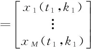
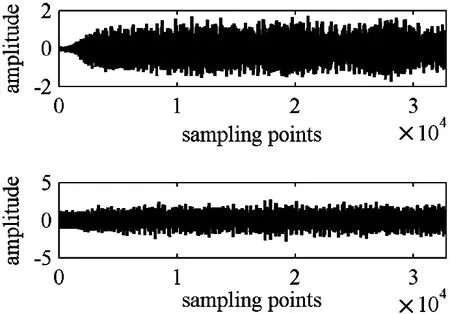
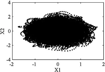
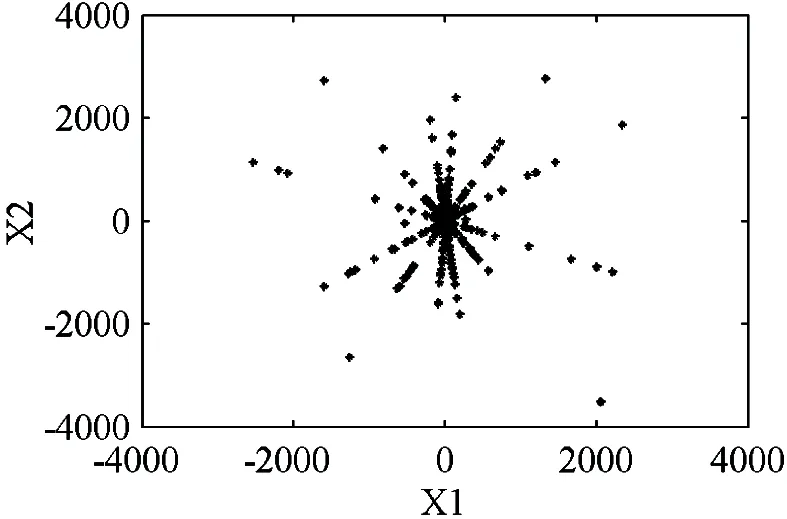
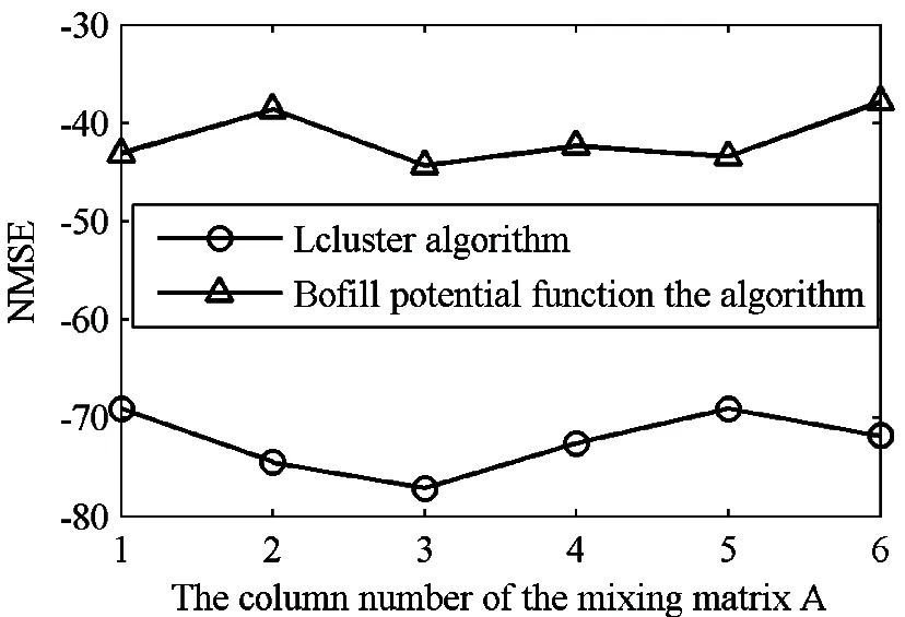
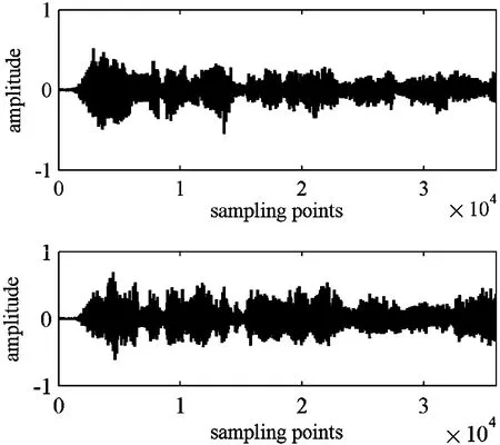
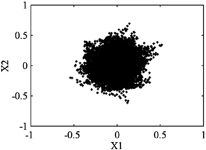
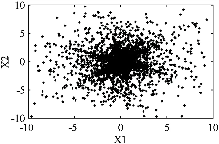
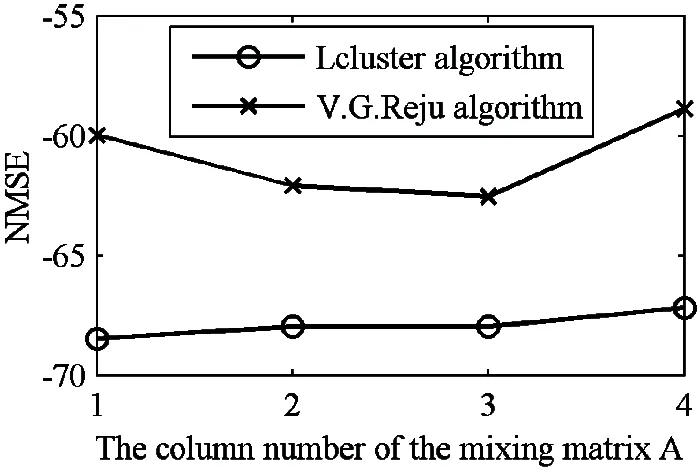
-∞ Parameter α is calculated as (6) Generally there is certain relationship between α and β in the following: (7) whereσis the standard deviation. From Eq.(7) it concludes that the GGD probability density function actually is determined only by shape parameter α. Studies show when α infinitely approximates zero, the GGD probability density function is approximate to δ function which indicates a strong sparse signal; whenαis equal to 1, GGD is degraded into Laplacian distribution, which is a sparse signal; when α is equal to 2, GGD is further degraded into Gaussian distribution and signal’s sparsity becomes unapparent; and whenαapproaches +∞, GGD tends to uniform distribution infinitely, which is a non-sparse signal. Therefore, the smaller the shape parameter α is, the sparser the signal is and the stronger the linear aggregation is. One of requirement of UBSS is independent of each other, actually it is difficult to ensure the signals are completely independent in practical situations. The signal linearity degree is influenced not only by sparse linear extent but also by the signal’s independence. The traditional independence between signals is defined by the probability density function. However this work studies the signals correlation combined with the entropy of information theory, and defines center entropy on the basis of the center of the signal related to the independence and the entropy measure[22]. Center entropy is defined as the center of the correlation: (8) γ(X,Y)=max(|u(X,Y)|, |u(-X,Y)|) (9) The center corr-entropy γ is a large value, which means that the relevance of the signals is weak and the signal is of stronger independence; similarly γ is a small value, which means that the signals relevance is stronger and the signal is of weaker independence. If the signals have stronger independence, its center corr-entropy is near to 1; and on the contrary weak independence means center corr-entropy near to 0. In summary, the center corr-entropy of signals is bigger and the shape parameter is smaller, which means that the linear aggregation degree of signals is stronger and there will have clear directional lines in scatter plot. The center corr-entropy of signals is smaller and the shape parameter is bigger, which means that the linear aggregation degree of signals is weaker and the scatter plot showing directional blur even without showing directionality. Therefore, shape parameter α and center corr-entropy γ can be used to measure signals linear aggregation degree. Mixing matrix A can be estimated directly using the clustering method with the clear line direction of observation signals. On the contrary, A is estimated with large errors even can not be estimated with weak direction. Generally, many actual signals are not sparse in time domain and there appear certain but not enough sparsity in the transformation domain which results in obscurely linear aggregation. This study proposes to detect and choose the transformation coefficients of time-frequency domain and it results in strong linear aggregation. 3.1 Enhance linear aggregation based on linear coefficients Eq.(1) is processed by short-time Fourier transform (STFT) and it obtains the following: (10) Assume that only source signal s1(t1,k1) is non-zero on a certain (t1,k1) in time-frequency domain while the other signals are all zero, then there exists: (11) Respectively dividing the real and imaginary components of any two observed signals in Eq.(11) and the following ratio is obtained: (12) where i∈M, j∈M, and i≠j. It can conclude that the ratios ai1/aj1between the real and imaginary components of any two observed signals are equal and at the same direction with column vector of mixing matrix. Similarly in other case of only single source signal, the ratios between the real and imaginary components of any two observed signals would also be equal. More generally, it is assumed that the ratio of theithcolumn of the mixing matrix A is equal to the ratio of coefficients which aggregates on theithcolumn of mixing matrix in time frequency point (tZ,kZ). So Eq.(13) is got: (13) The simplest case of Eq.(13) is that only one signal source presents while other source signals are inactive or offsetting each other at point (tZ,kZ) Eq.(13) can be written as (14) It can conclude from Eq. (14) that the ratio of coefficient real component is equal to the imaginary component radio as well as the ratio of mixing matrix corresponds column. Consequently, it can define these coefficients as linear coefficients which have strong linear aggregation in the time-frequency domain and can exhibits distinct directionality in the scatter plot. This work enhanced linear aggregation degree based on the linear coefficients. However, actually the values of Re[Xi(t,k)]/Re[Xj(t,k)] and lm[Xi(t,k)]/lm[Xj(t,k)] in Eq.(12) are not completely equal and certain discrepancies exist between these values. Considering the actual feasibility, threshold value ω is set and Eq.(13) can be expressed as (15) whereωis an empirical value with a range of (0, 0.1) which is modified according to the signals. After linear coefficients process, the linear aggregation of observation signals is enhanced. 3.2 Mixing matrix estimation Assume that M=2, these linear coefficients are subject to unitization processed by Eq.(16) and a setUis obtained: (16) where X(tZ,kZ) is the linear coefficient selected from time-frequency domain, and ΩZis a set of all selected linear coefficients. These vectors in ΩZare all unit vectors, and by further calculating the ratios among the vectors it obtains a set H: (17) The setHis classified by clustering method and if any twohm,hninHare equal or approximately equal, they are classified into same category. (18) where sum(Cn) is the number of all vectors in thenthcategory, ∑hCnis the sum of all elements in thenthcategory. The estimation of mixing matrix column vectors is achieved by (19) The proposed method is used to process three different cases which belong to UBSS and the simulation results and analysis are presented. The normalized mean square error (NMSE) is applied to evaluate the mixing matrix accuracy and the comparisons with other methods are also presented. The normalized mean square error is defined as (20) (1) Strong linear aggregation, i.e. shape parameter α and correlation coefficient r are small: Consider the case: M=2 and N=6, which means six source signals and two observation signals. The six source signals are intercepted from flute acoustical signals of Bofill’s study[23]and sampling points are 32768. Mixing matrix A is generated randomly, and its column vectors are normalized as: A= Fig.1 Waveform of observation signals in the time domain Obeying the generalized Gaussian distribution, shape parameter α and correlation coefficient r of two observation signals are calculated in the time domain (TD) and time-frequency domain (TFD), respectively, and the result is shown in Table 1. Table 1 Shape parameter and correlation coefficient Table 1 shows that shape parameter α is greater than two in TD and becomes small in TFD, and correlation coefficient of the two observed signals is small. Therefore it concludes that observation signals will present strong linear aggregation and distinct directionality in time-frequency domain. Fig.2 illustrates the conclusion: (1) is scatter plot of transformation coefficients in TD and (2) is scatter plot of linear coefficients in TFD. (a) Scatter plot in TD (b) Scatter plot in TFD Fig.2 verifies the conclusions and therefore mixing matrix A can be estimated directly using improved K-means clustering algorithm and it can obtain the estimation result: Fig.3 NMSE comparison of Bofill’s and Lcluster algorithm Fig.3 shows that NMSE of estimation by the proposed algorithm is significantly smaller than that by Bofill potential function algorithm. (2) Weak linear aggregation, i.e. large shape parameter α and small correlation coefficient r: Consider the case: M=2 and N=4, i.e. four source signals and two observed signals. The four source signals are actual speech signals from http://www.speech.cs.cmu.edu/cmu_arctic/. The sampling points of each source signals are 35920, and the mixing matrix is The two observation signals are generated according to Eq.(1) and shown in Fig.4. Fig.4 Waveform of observation signals in time domain Obeying the generalized Gaussian distribution, shape parameter α and correlation coefficient r of two observation signals are calculated in TD and TFD, respectively, and the result was shown in Table 2. Table 2 Shape parameter and correlation coefficient It can be seen from Table 2 that the correlation coefficient is small,while the shape parameter is not sufficiently small both in TD and in TFD, So it is deduced that the signals will present weak linear aggregation in the TFD. Fig.5 includes scatter plots of two observation signals in TD and TFD, respectively. (a) Scatter plot in TD (b) Scatter plot in TFD Fig.5(b) shows that the scatter plot of observation signals presented obscure directivity in TFD and the conclusion is verified by Fig.5. The linear coefficients in TFD are selected according to Eq.(16), whereinωwas selected as 0.025. The scatter plot of linear coefficients is shown in Fig.6. These linear coefficients are used to estimate mixing matrix in accordance with the proposed method in Section 4.2 and obtain the estimated value of mixing matrix: Fig.7 NMSE comparison with Lcluster and VG.Reju algorithm Simulation shows that NMSE of estimated mixing matrix by proposed algorithm is significantly smaller than that by V.G.Reju algorithm. This study investigates the mixing matrix estimation under UBSS by studying the linear aggregation characteristic and correlation effect of observation signals. In order to accurately estimate the mixing matrix with unknown sparsity, the relationship between shape parameter and sparsity of observation signals following the generalized Gaussian distribution is studied. The effects of shape parameter and correlation coefficient of the observed signals on the linear aggregation character is focussed, and then the specific processing algorithms aimed at different linear aggregations are adopted. The mixing matrix can be estimated directly using the improved K-means algorithm if the linear aggregation is strong; on the contrary, mixing matrix is estimated by selecting the appropriate single source coefficients based on linear coefficients before applying the improved K-means. Experiment results show that the proposed method can effectively estimate the mixing matrix with different sparsity while retaining the characteristics of low computational complexity and high estimation accuracy. Reference [ 1] Li Y Q, Wang J. Sequential blind extraction of instantaneously mixed sources.IEEETransactiononSignalProcessing, 2002, 50(5): 997-1006 [ 2] Zhang L, Cichocki A, Amari S. Self-adaptive blind source separation based on activation function adaptation.IEEETransactiononNeuralNetworks, 2004, 15(2): 233-244 [ 3] Fadili J M, Starck J L, Bobin J, et al. Image decomposition and separation using sparse representations: an overview.ProceedingsoftheIEEE, 2010, 98(6): 983-994 [ 4] Ma J, Huang G M, Zuo W. A robust underdetermined blind sources separation algorithm for ill-conditioned mixing signals.JournalofElectronics&InformationTechnology, 2013, 35(10): 2379-2383 [ 5] Wei Z, Ju L, Sun J D, et al. A new two-stage approach to underdetermined blind source separation using sparse representation acoustics.SpeechandSignalProcessing, 2007, 3(3): 953-956 [ 6] Xie S L, Fu Y L. Searching-and-averaging method of underdetermined blind speech signal separation in time domain.ScienceinChinaSeriesF:informationScience, 2007, 50(5): 771-782 [ 7] Xie S L, Yang L,Yang J M, et al. Time-frequency approach to underdetermined blind source separation.IEEETransactionsonNeuralNetworksandLearningSystems, 2012, 23(2): 306-316 [ 8] Fang Y, Zhang Y, A robust clustering algorithm for underdetermined blind separation of sparse sources.JournalofShanghaiUniversity(EnglishEdition), 2008, 12(3): 228-234 [ 9] Tazehkand B M, Tinati M A. Underdetermined blind mixing matrix estimation using STWP analysis for speech source signals.WirelessSensorNetwork, 2010, 2(1): 854-860 [10] Lee T W, Lewicki M S, Girolami M. Blind source separation of more sources than mixtures using overcomplete representations.IEEESignalProcessingLetters, 1999, 6(4): 87-90 [11] Frigui H, Krishnapuram R. A robust algorithm for automatic extraction of an unknown number of cluster from noisy data.PatternRecognitionLetter, 1996, 17(12): 1223-1232 [12] Grady P D O, Pearlmutter B A. The LOST algorithm: finding lines and separating speech mixtures.EURASIPJ.Adv.SignalProcess, 2008, 12(2): 784296-1-784296-19 [13] Lv Q, Zhang X D. A unified method for blind separation of sparse sources with unknown source number.IEEESignalProcessLetter, 2006, 3(1): 49-51 [14] Li Y, Cichocki A, Amari S. Analysis of sparse representation and blind source separation.NeuralComputation, 2004, 16(6): 1193-1234 [15] Yilmaz O, Rickard S. Blind separation of speech mixtures via time-frequency masking.IEEETranactiononSignalProcessing, 2004, 52(7): 1830-1847 [16] Abrard F, Deville Y. A time-frequency blind signal separation method applicable to underdetermined mixtures of dependent sources.SignalProcessing, 2005, 85(7): 211-221 [17] Jayaraman J, Thiagarajan. Mixing matrix estimation using discriminative clustering for blind source separation.DigitalSignalProcessing, 2013, 23(1): 9-18 [18] Zhou G X, Yang Z Y, Xie S L. Mixing matrix estimation from sparse mixtures with unknown number of source.IEEETrans.NeuralNetworks, 2011, 22(2): 211-221 [19] He Z S, Xie S L, Fu Y L. Sparse analysis of signals.ProgressinNaturalScience, 2006, 16(9): 1167-1173 [20] Dong T B, Lei Y K, J S Yang. An algorithm for underdetermined mixing matrix estimation.Neurocomputing, 2013, 3(15): 26-34 [21] Leydold J, Homann W. Generating generalized inverse Gaussian random variates by fast inversion.ComputationalStatistics&DataAnalysis, 55 (1) (2011) 213-217 [22] Ou S F, Zhao X H, Gao Y. Adaptive combination algorithm and its modified scheme for blind source separation.JournalofElectronics&InformationTechnology, 2011, 33(5): 1243-1247 [23] Bofill P, Zibulevesky M. Undetermined blind source separation using sparse representations.Signalprocessing, 2001, 81(11): 2353-2362 [24] Washizawa Y, Cichocki A. Sparse blind identification and separation by using adaptive K-orthodrome clustering.Neurocomputing, 2008, 71 (10): 2321-2329 [25] Reju V G, Soo Ngee Koh, Ing Yann Soon. An algorithm for mixing matrix estimation in instantaneous blind source separation.SignalProcessing, 2009, 89: 1762-1773 Wen Jiangtao, born in 1974. He received his Ph.D degree in Department of Precision Instrument of Tsinghua University in 2009. He also received his B.S. and M.S. degrees from Yanshan University in 1998 and 2003 respectively. Now he is an Associate Professor in School of Electrical Engineering, Yanshan University. His research interests include blind source separation and application, complex vibration signal processing and pattern recognition. 10.3772/j.issn.1006-6748.2016.01.012 ① Supported by the National Natural Science Foundation of China (No. 51204145) and Natural Science Foundation of Hebei Province of China(No. 2013203300). ② To whom correspondence should be addressed. E-mail: wjtsjd@163.comReceived on June, 16, 2015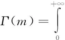


3 Mixing matrix estimation under weak linear aggregation

4 Algorithm simulation and result analysis








5 Conclusions
 High Technology Letters2016年1期
- High Technology Letters的其它文章
- An effective estimation of distribution algorithm for parallel litho machine scheduling with reticle constraints①
- Selective transmission and channel estimation in massive MIMO systems①
- Time difference based measurement of ultrasonic cavitations in wastewater treatment①
- Robust SLAM using square-root cubature Kalman filter and Huber’s GM-estimator①
- An improved potential field method for mobile robot navigation①
- Research on the adaptive hybrid search tree anti-collision algorithm in RFID system①
