Income smoothing and the cost of debt

Si Li，Nivine Richie

aWilfrid Laurier University，Lazaridis School of Business and Economics，Canada

bUniversity of North Carolina Wilmington，United States

Income smoothing and the cost of debt

Si Lia，1，Nivine Richieb，*

aWilfrid Laurier University，Lazaridis School of Business and Economics，Canada

bUniversity of North Carolina Wilmington，United States

A R T I C L EI N F O

Article history:

Accepted 28 March 2016

Available online 4 May 2016

JEL classification:

G-12

G-32

Income smoothing

Earnings smoothing

Cost of debt

Credit spreads

Credit ratings

Garbling

The literature on income smoothing focuses on the effect of earnings smoothing on the equity market.This paper investigates the effect of income smoothing on the debt market.Using the Tucker-Zarowin（TZ）statistic of income smoothing，we find that firms with higher income smoothing rankings exhibit lower cost of debt，suggesting that the information signaling effect of income smoothing dominates the garbling effect.We also find that the effect of earnings smoothing on debt cost reduction is stronger in firms with more opaque information and greater distress risk.

©2016 Sun Yat-sen University.Production and hosting by Elsevier B.V.This is an open access article under the CC BY-NC-ND license（http://creativecommons.org/licenses/by-nc-nd/4.0/）.

1.Introduction

Although income smoothing has existed for decades，there is limited academic research on earnings smoothing.For example，Graham et al.（2005）report that‘‘an overwhelming 96.9%of the survey respondents indicate that they prefer a smooth earnings path.Such a strong enthusiasm among managers for smooth earnings is perhaps not reflected in the academic literature.”More recently，Dichev et al.（2013）state that‘‘earnings management is driven by a host of intertwined factors but capital market motivations dominate，followed by debt contracting，and career and compensation issues.”

There are generally two schools of thought as to what motivates managers to smooth.First，smoothing presents an arguably efficient vehicle for managers to reveal private information because it is easier for investors to predict future earnings from smoother earnings.Second，smoothing represents‘‘garbling”；that is，smoothing is an exercise undertaken by managers in an attempt to fool analysts and others and to enhance managerial careers or compensation.The first school of thought（the information signaling view）is reflected in the works of Ronen and Sadan（1981），Demski（1998），Sankar and Subramanyam（2001），Srinidhi et al.（2001），Kirschenheiter and Melumad（2002）and Goel（2003），among others.Essentially，this school holds that income smoothing may reveal private information in much the same way that dividend smoothing can lead to information revelation（Miller and Rock，1985）.The second school of thought（the information garbling view）is reflected in the works of Beidleman（1973），Lambert（1984），Healy（1985），Fudenberg and Tirole（1995），Arya et al.（1998）and Demski and Frimor（1999），among others.

A handful of empirical studies have investigated the issue of income smoothing in the context of equity markets.Subramanyam（1996）finds that stock returns are positively associated with contemporaneous discretionary accruals，which are a measure of income smoothing.Hunt et al.（2000）find that income smoothing improves price-earnings multiples.Tucker and Zarowin（2006）report that the changes in the current stock prices of higher smoothing firms contain more information about these firms'future earnings than do the changes in the current stock prices of lower smoothing firms.Taken collectively，these studies support the notion that income smoothing represents an efficient vehicle for managers to reveal private information.Using survey data，Graham et al.（2005）find that the overwhelming majority of managers prefer a smooth earnings growth rate.2As far as we know，there is no direct empirical evidence for how earnings smoothing affects the cost of equity capital.The accounting literature does provide evidence that earnings management（as measured by accrual quality）‘‘is frequently considered to increase opacity，decrease liquidity and increase equity cost of capital”（Lang and Maffett，2011）.

Instead of examining the effect of income smoothing on the equity market，our paper examines the effect of income smoothing on the credit market.If income smoothing is informative and mitigates the asymmetric information problem between the firm and investors，then smoothing firms may exhibit a lower cost of debt capital due to lower information risk.This idea follows from the theory in Trueman and Titman（1988），who argue that a smooth earnings stream may potentially decrease assessments of default risk，and thus decrease the debt cost of capital.However，if income smoothing is garbling，and creditors can recognize smoothing as garbling，then smoothing firms could exhibit a higher cost of debt capital as creditors punish managers for gaming earnings.

Investigating the credit market is of great interest for the following reasons.First，investors in the bond market are predominantly institutional investors.For example，transactions with less than$1 million face value are considered‘‘odd lots”（that is，less than the normal unit of trading）.Because creditors are typically professional investors，they may be more able than equity stakeholders to differentiate the information effect from the garbling effect.Therefore，examining the signaling versus garbling debate through the lens of credit markets can help enhance our understanding of earnings smoothing.Second，Lang and Maffett（2011）argue that firm-level transparency could affect equity and debt differently.They mention that‘‘Earnings smoothing is likely to be a particular issue...given the importance of stakeholders other than equity investors.In particular，stakeholders such as labor unions，governments and debt holders are exposed more directly to losses than to gains and so prefer lower risk.As a consequence，managers have incentives to report smooth earnings to create the impression of a less risky earnings stream.”Managers have incentives to signal to the market to obtain debt financing at a lower cost because，all else being equal，lower debt costs imply more money left for shareholders and managers.

In addition to contributing to the literature on incoming smoothing，this study is related to extant studies that identify the determinants of the cost of debt.For example，Chen et al.（2007）report that bond liquidity is an important factor in explaining corporate yield spreads.Tang and Yan（2006）document liquidity effects with respect to credit default swap spreads.Our research suggests that income smoothing could serve as an additional factor that determines the cost of debt，as measured by credit spreads.Finally，this study is related to a growing body of research that addresses the issue of accounting transparency and asset pricing.In this context，the research presented here is perhaps most closely related to Yu（2005），who finds that firms withmore information disclosure（measured as AIMR disclosure rankings）tend to exhibit lower credit spreads.3‘‘AIMR”stands for the Association for Investment Management and Research，the former name of the CFA Institute.Yu's（2005）findings are consistent with the theory of discretionary disclosure that began with Verrecchia（1983），and with the incomplete accounting information model of Duffie and Lando（2001）.By examining income smoothing，our paper provides evidence for whether income smoothing enhances（or reduces）the quality of information disclosure，which can be further translated into lower（or higher）cost of debt.

Using a large sample of publicly traded companies and the Tucker and Zarowin（2006）measure of income smoothing，we examine whether higher smoothing firms witness higher or lower cost of debt than their lower smoothing counterparts.The results indicate that higher smoothing firms exhibit lower cost of debt，both unconditionally and after controlling for factors previously known to explain credit spreads.Our results further suggest that the information signaling effect of income smoothing in reducing the cost of debt is stronger in firms with more opaque information，such as smaller firms.The effect is also stronger in firms with more distress risk，such as more volatile，less profitable and lower credit rating firms.Assuming that creditors are not fooled by income smoothing，the evidence presented here from the credit market affirms the conclusion drawn from most of the existing research using equity market data，namely that income smoothing may aid management to revel private information.

2.Research design

2.1.Measuring income smoothing

Income smoothing is commonly understood to mean management's use of discretionary accounting and management principles to reduce earnings variability.The main income smoothing measure used in this study is the standard metric used in the literature.Following Myers and Skinner（2002），Leuz et al.（2003），and Tucker and Zarowin（2006），we estimate income smoothing as the negative correlation between the change in a firm's discretionary-accruals proxy（ΔDAP）and the change in its pre-discretionary income（ΔPDI）.This measure assumes that there is an innate，un-managed income series and that management uses discretionary accruals to smooth this raw series.When there is an increase（decrease）in the pre-discretionary income，a firm will use negative（positive）discretionary accruals to smooth its earnings.As a result，income smoothing is presented as the negative correlation between ΔDAP and ΔPDI，and more income smoothing is evidenced by a greater degree of negative correlation between ΔDAP and ΔPDI.

To estimate discretionary accruals，we follow Tucker and Zarowin（2006）by using the cross-sectional version of the Jones（1991）model as modified by Kothari et al.（2005），namely:

where ASSETS is total assets；ACCRUALS stands for total accruals estimated as net income minus operating cash flows，deflated by lagged total assets；ΔSALES is change in sales scaled by lagged total assets；and PPE is gross property，plant and equipment scaled by lagged total assets.4Data definitions and measurement details for all of the variables are reported in the Appendix.ROA，return on assets，is measured as net income over lagged total assets.Following Tucker and Zarowin（2006），we include ROA in the regression because previous research finds that the Jones model is misspecified for well-performing or poorly performing firms（see Dechow et al.，1995 and Kothari et al.，2005）.We also follow Tucker and Zarowin（2006）and omit a separate intercept term in regression（1）.We perform a robustness analysis by estimating regression（1）with an intercept term，as in Eq.（7）of Kothari et al.（2005），and obtain similar results.

Non-discretionary accruals（NDAP）of firm j are then represented by the fitted values of regression（1）:

Discretionary accruals（DAP）are represented by the residuals，that is，the deviations of actual accruals from NDAP.The un-managed income series，i.e.，pre-discretionary income（PDI），is calculated as net income（NI）minus discretionary accruals，or PDI=NI-DAP.Note that as DAP is assets-scaled，NI should also be assets-scaled here.

Table 1Estimation of discretionary accruals and income smoothing.

The regression is estimated using all of the firms in the same industry（two-digit SIC）for each year，using annual data for the 1988-2007 period.There are 951 industry-year regressions and the obtained estimates are summarized in the following table.ACCRUALS，ΔSALES，PPE and ROA are scaled by lagged assets.Panel B reports the summary statistics of the income smoothing measures in which discretionary accruals is DAP and pre-discretionary income（PDI）=Net income（NI）-DAP.Detailed definitions of the variables are reported in the Appendix.

The smoothing measure is estimated as the correlation between the change in discretionary accruals and the change in un-managed income，Corr（ΔDAP，ΔPDI），using the current year's and past four years'observations.Firms with more negative correlations are higher smoothing firms，whereas firms with less negative（or positive）correlations are lower smoothing firms.For ease of interpretation，we follow Tucker and Zarowin（2006）in creating our final income smoothing measure（IS），by converting the correlations into reverse fractional rankings by 2-digit industry SIC code.The IS measure ranges from 0 to 1 by industryyear with the highest income smoothers（most negative correlations）having high rankings and lowest income smoothers（less negative correlations）having low rankings.

We estimate regression（1）using all of the firms in the same industry（two-digit SIC）each year for the 1988 to 2007 period.We obtain the information on the variables from Compustat.Our sample starts in 1988 because one key variable that is used to estimate accruals，cash flow from operations，is only available from Compustat after 1988.Our sample stops just prior to the credit crisis that began in 2008.Because this study relies heavily on credit market data，we have chosen to avoid the issues associated with illiquidity and lack of reliable bond pricing that existed beginning in 2008.We exclude all of the firms in SIC codes 4000-4999（regulated industries）and 6000-6999（financial industries）because firms in these industries may have distinct types of accounting and debt costs.We then sort the sample firms by 2-digit SIC category per year.We discard any cross-section with less than 10 firms per industry-year category，resulting in 951 industry-year cross sections.Following the literature（Tucker and Zarowin，2006），we Winsorize the variables used in Eq.（1）at±three standard deviations per year.5We also Winsorize at±three standard deviations per industry-year and find the results are qualitatively similar.

To show that our income smoothing estimates are in line with those presented in the literature，we first provide the regression（1）estimation results in Table 1 Panel A and show that the main statistics of the coefficient estimates in the accruals equation are comparable to those reported by Subramanyam（1996）and Tucker and Zarowin（2006）.In addition，similar to Tucker and Zarowin（2006），we find that the mean coefficient on ROA is 0.501，indicating that accruals are positively related to profitability.

Table 1 Panel B presents the summary statistics of income smoothing variables in our sample.The earnings smoothing correlation Corr（ΔDAP，ΔPDI）is-0.731，on average，with a median value of-0.922，which isconsistent with the mean and median reported by Tucker and Zarowin（2006）of-0.709 and-0.899，respectively.

2.2.Estimating the cost of debt

In an effort to improve bond market transparency，the National Association of Securities Dealers（NASD）began collecting and reporting bond transaction data in July 2002，using the Trade Reporting and Compliance Engine（TRACE）.The TRACE system is designed to allow NASD members to‘‘report over-the-counter（OTC）secondary market transactions in eligible fixed income securities to NASD and subject certain transaction reports to dissemination.”6In July 2007，the NASD and the member regulation，enforcement and arbitrage functions of the NYSE were consolidated to form the Financial Industry Regulatory Authority（FINRA）.The history of the TRACE system is available online at www.finra.org/compliance/ MarketTransparency/TRACE/FAQ/P085430.The Trade Reporting and Compliance Engine is the FINRA-developed vehicle that facilitates the mandatory reporting of over-the-counter secondary market transactions in eligible fixed income securities.All of the broker/dealers who are FINRA member firms have an obligation to report transactions in corporate bonds to TRACE under a SEC-approved set of rules.The system captures and disseminates consolidated information on secondary market transactions in publicly traded TRACE-eligible securities（investment grade，high yield and convertible corporate debt）representing all of the over-the-counter market activity in these bonds.The original TRACE-eligible securities included 500 corporate bonds of which 50 were high-yield securities.Currently，transaction data are reported for over 4000 different bond issues with approximately 20 percent of those issues being high-yield securities.

We use TRACE data to estimate the cost of debt for our sample of publicly traded firms from July 2002 through December 2007.The data are cleaned by eliminating all of the canceled or corrected trades，whether the cancellation is entered on the same transaction date or entered on a different transaction date.7Based on TRACE documentation，trade errors that are caught the same trading day are corrected by entering a TRC_ST of C（cancellation）or W（correction or‘was'）.These corrections are coded with the original message sequence number to identify a corrected trade.If a trade error is caught after the trade date，then it is corrected by entering an ASOF_CD of R（reversal）and an A（as of trade）. These corrections are not linked to the original message sequence number so they must be matched based on trade date，time，price and volume.Occasionally，there is more than one original trade that matches a reversal，and occasionally there is more than one reversal trade for which no original trade can be found.We select the first matching original trade for each reversal and if no original trade can be found，then the reversal is assumed to be entered in error and is eliminated.We further clean the data by eliminating all of the‘‘when-issue”trades and all of the trades that do not settle regular way. We select trades where the price excludes commission and，following Edwards et al.（2007），where the trade size is greater than or equal to$100，000.We further use the information from the Fixed Investment Security Database（FISD）to limit the sample to U.S.dollar-denominated，senior corporate debt issues.We also exclude privately placed，putable，exchangeable，perpetual and preferred securities.As a large number of firms in our sample issue callable bonds，we include callable issues and substitute the call date for the maturity date if the call is in-the-money.The most appropriate way to identify whether a bond is likely to be called is to select bonds where the yield-to-call is lower than the yield-to-maturity.However，in the absence of yield-to-call data，we compare the coupon rate to the yield-to-maturity.If the yield-to-maturity is lower than the coupon rate，then we substitute the call date for the maturity date of the bond issue.To estimate a daily yield from the transaction data we use the mid-point of all of the trades during the day to reflect the day's yield.Our final sample consists of 796 unique firms and 2097 bond issues.

Matching the high frequency transaction data of TRACE with annual data from Compustat presents a challenge for our sampling frequency.This is further complicated by the fact that many firms have more than one bond issue being reported.Of the firms in our sample，359 have only one bond issue.The average number of bond issues per firm in our sample is 2.6 and the median is 2.The maximum number of issues per firm in our sample is 25.Bessembinder et al.（2008）describe three possible approaches to sampling bond data:（1）a representative bond approach，（2）a bond-level approach and（3）a firm-level approach.In the representative bond approach，researchers select one bond per firm，even though the firm may have several different bond issues outstanding.This approach faces serious limitations because different bond issues will have different durations；selecting one representative bond will necessarily ignore effects on other parts of the yield curve.The bond-level approach captures more information than the representative approach as it treats each bond as a separate observation.Although this is preferred to the representative approach，it is not without problems of its own.Bessembinder et al.（2008）point out that this approach faces correlations across observations within the firm，and thus may weight higher quality firms more heavily as they are more likely to have multiple bond issues.The firm-level approach uses a market-value weighted average yield of all of the bonds per day per firm as the cost of debt capital.This composite measure of the cost of debt is free from the cross-correlation problem of the bond-level approach.In our study，we present results for both the bond-level and firm-level approaches.

3.Univariate analysis

Using the TZ earnings smoothing statistic，we perform a univariate analysis of the characteristics of high and low smoothing firms over the 2002-2007 sample period.Table 2 presents the results from comparing the top quartile with the bottom quartile（based on the TZ statistic）of the sample firms.By definition，the high smoothing firms have more negative TZ statistics with a mean of-0.99，whereas the low smoothing firms have less negative TZ statistics with a mean of-0.60.

Table 2 Panel A shows that the sample firms with smoother earnings are larger，more profitable，have more operating cash flows and have more growth options，than the firms with less smooth earnings.Higher smoothing firms have significantly lower debt-to-asset ratios—26 percent，on average，compared with lower smoothing firms with 37 percent，on average.The Z-score for the higher smoothing firms is significantly higher than for low smoothing firms，indicating that higher smoothing firms are financially healthier.Therefore，we control for all of these firm characteristics in our multivariate analysis.In addition，the statistics show that firms with smoother earnings also engage in more earnings management，as measured by the absolute value of discretionary accruals，DAP，estimated as the residual from regression（1）.This suggests that income smoothing is related to earnings management.Indeed，we find that the reverse rank of TZ statistic and the absolute value of DAP are positively correlated at 0.15.

Table 2 Panel B shows that the high smoothing firms have lower average bond yields and higher average bond ratings than their low smoothing counterparts.The average bond yield for high smoothing firms is 5.35 percent，whereas the average bond yield for low smoothing firms is 6.78 percent，and this difference is statistically significant at conventional levels.Likewise，the average bond rating for high smoothing firms is 6.9（approximately A-where the scale begins at 1 for AAA，2 for AA+，...，and 22 for D）.The average bond rating for low smoothing firms is 11.14，which corresponds to a BB+rating.In addition，the bonds issued by top smoothing firms exhibit shorter terms to maturity and terms to call，lower coupon rates and higher amounts outstanding.In our subsequent multivariate regressions，we control for the above bond characteristics. Overall，these univariate results provide preliminary evidence that firms which smooth earnings have lower cost of debt，suggesting that they are signaling rather than garbling earnings information.

4.Multivariate analysis

4.1.Baseline regressions

We now turn to a multivariate analysis of the cost of debt capital by estimating a pooled cross-sectional time-series model using both a bond-level approach and a firm-level approach.The dependent variable is the daily yield per bond（bond-level approach）or the weighted average daily yield per firm（firm-level approach）.The key explanatory variable is the income smoothing ranking（IS），which we expect to have a positive coefficient in the case of garbling and a negative coefficient in the case of signaling.The control variables are included based on prior research，which indicates the variables'explanatory power on cost of debt capital.Some of the control variables with predicted signs are described below.

4.1.1.Firm-specific factors

We first control for various firm characteristics，such as size，growth，profitability，Zscore and tangibility. These control variables deal with potential endogeneity；specifically，that firms with certain characteristics maybe associated with higher or lower cost of debt，and that these characteristics are correlated with income smoothing.For example，Ronen and Sadan（1981）use a signaling model and contend that only firms with good prospects elect to smooth.We discuss some of the following firm level control variables.

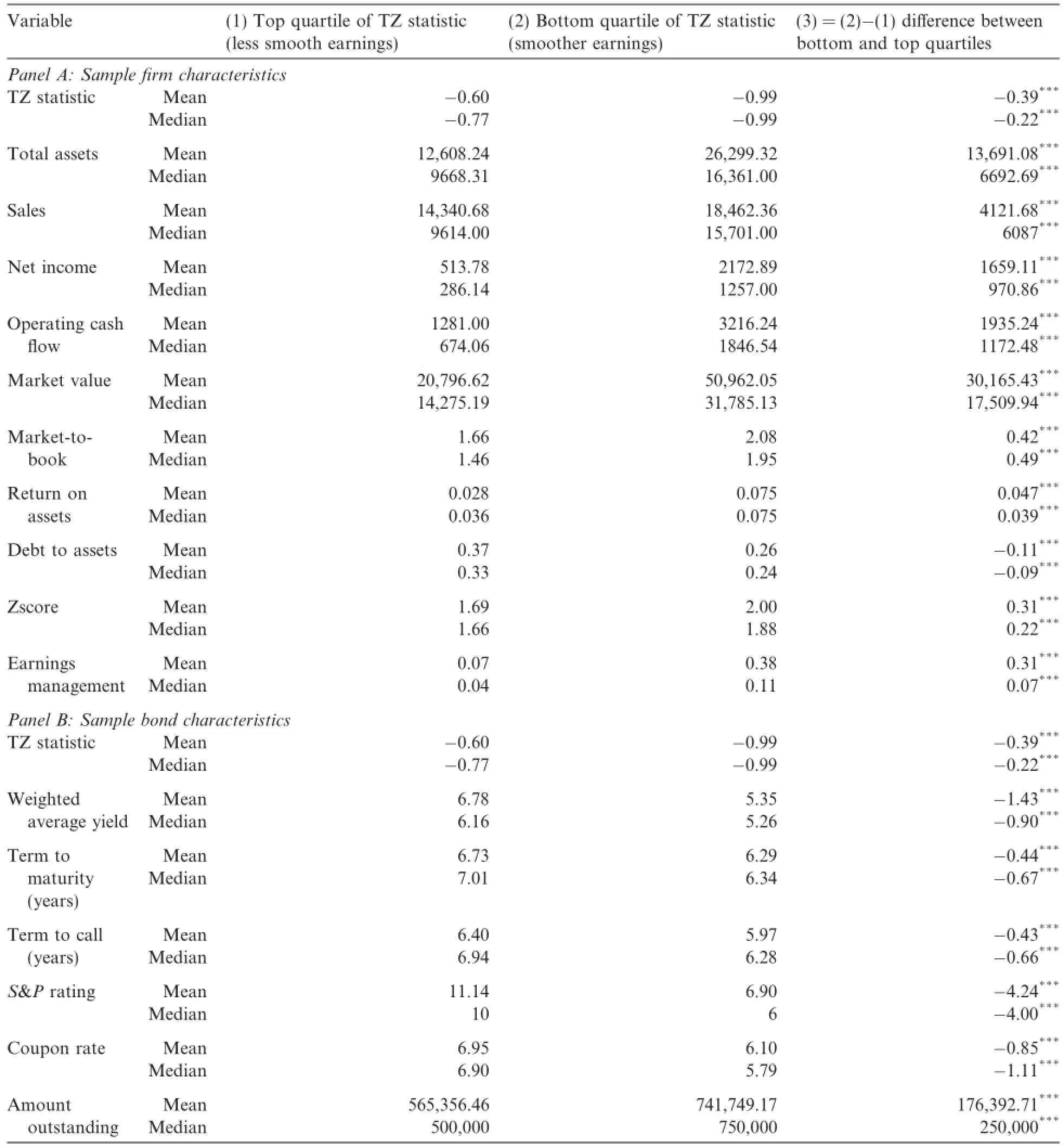
Table 2Univariate analysis.

·Sales revenue to proxy for firm size，as larger firms can have economies of scale that would serve to reduce credit spreads（predicted negative sign）.8Sales revenue may also proxy for instrument liquidity（an instrument-specific factor），as it may reflect firm size and therefore issue size. Issue size is an often-used proxy for bond liquidity（Yu，2005）.

·Return on assets，which is a proxy for profitability as more profitable firms will have lower credit spreads（predicted negative sign）.

·Firm volatility，with higher volatility implying higher default risk and thus higher credit spreads（predicted positive sign）.

·Market-to-book ratio，where market value is the market value of equity plus the book value of debt and book value is the book value of assets.This is to control for differences in investment opportunities，with higher ratios implying either higher or lower credit spreads.High growth firms have more growth opportunities and this may be related to lower debt cost.In contrast，high growth option firms may have more intangibles and thus few tangibles in the company and this is related to higher debt costs（sign ambiguous）.

4.1.2.Instrument-specific factors

·Bond coupon，which is a proxy for any tax effects（sign ambiguous）.

·Illiquidity，following Chen et al.（2007），who find that less liquid issues are associated with higher bond yield spreads（predicted positive sign）.

4.1.3.Market or macroeconomic factors

The literature suggests that credit spread and term spread are good proxies of macroeconomic conditions and help explain stock and bond returns（Chen et al.，1986；Fama and French，1993）.Specifically，credit spreads tend to widen in recessions and shrink in expansions（Collin-Dufresne et al.，2001），as investors require more compensation for increased default risk in bad economic times.High（low）term spreads are often used as an indicator of good（bad）economic prospects.As a result，we use the following two variables to proxy for macroeconomic conditions.

·Term spread is the slope of the prevailing treasury yield curve，often measured by the difference between

10-and 2-year treasury bond yields（predicted negative sign）.

·Credit spread is the slope of the corporate debt yield curve，measured as the difference in yields between

AAA corporate bond yields and BAA corporate bond yields（predicted positive sign）.

Our complete model is estimated as

where AVEYIELD is the median daily yield per bond as reported by TRACE or the average of the median daily yield across all of the bond issues per firm；IS is the income smoothing ranking following Tucker and Zarowin（2006）；SIZE is the natural logarithm of beginning of period net sales；DEBT is the beginning of period ratio of total debt to total assets；ROA is the beginning of period net income over total assets；VOLAT isthe beginning of period standard deviation of CRSP daily equity returns using 252 days prior to bond spread measurements；MKBK is the beginning of period ratio of market value of the equity plus the book value of the debt to book value of the assets；COVERAGE is a dummy variable that takes a value of 1 if operating cash flows are greater than current liabilities；TANGIB is beginning of period property plant and equipment over total assets；ZSCORE is Altman's Z score；CALL is a dummy variable taking a value of 1 if the bond iscallable；lnMAT is the natural logarithm of the bond maturity measured in months（the natural log of the term to call is substituted if the bond call is in the money）；COUPON is the annual coupon rate of the bond；SP is the S&P credit rating converted to a numeric scale，where 1 represents AAA and 22 represents a rating of D；ILLIQ is the standard deviation of the price during the week divided by the total volume traded during the week；lnOUTST is the natural logarithm of the amount of bonds outstanding；TSPREAD is the term spread estimated as the difference between the 10-year treasury yield and the 2-year treasury yield as reported by the Federal Reserve Board of Governors；and CSPREAD is the credit spread estimated as the difference between AAA corporate bond yields and BAA corporate bond yields as reported by the Federal Reserve Board of Governors.

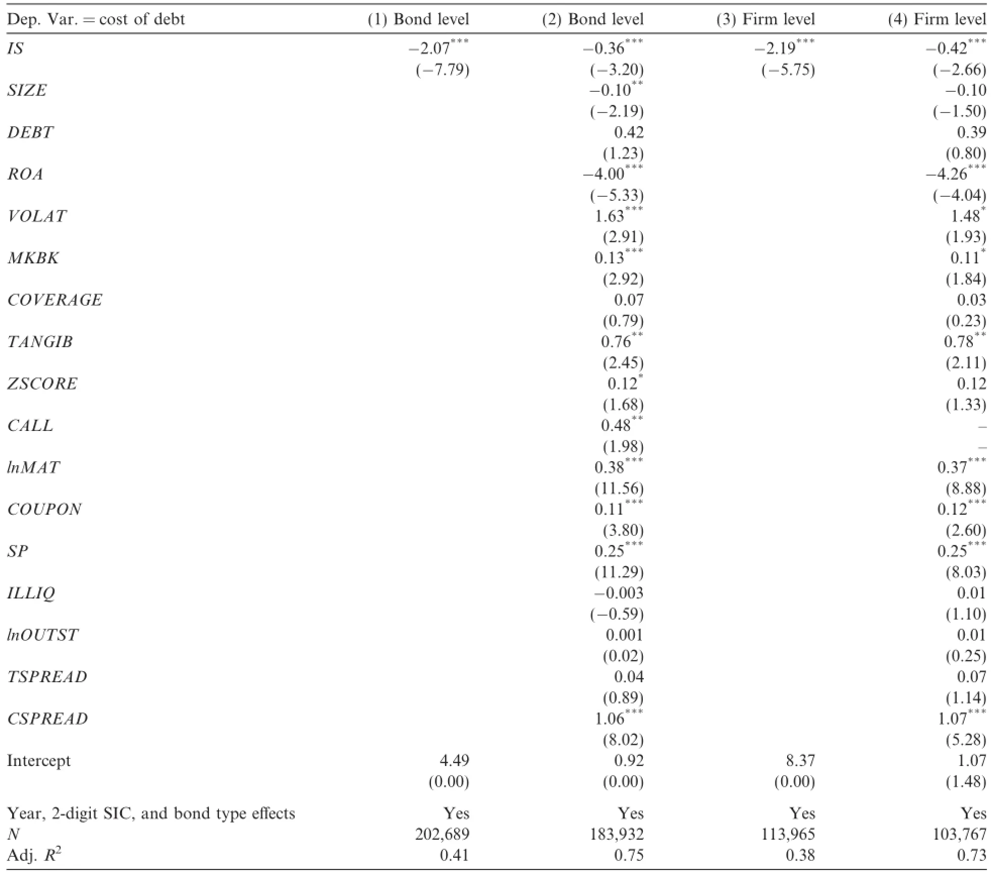
Table 3Effect of income smoothing on the cost of debt.

Table 3 presents the results of the baseline regression results.Columns（1）and（2）include bond-level regressions and Columns 3 and 4 include firm-level regressions.Consistent with our univariate analysis，the coefficients on IS in all four columns are negative and significant，indicating that higher earnings smoothing firms are associated with lower cost of debt.To illustrate the economic significance，we take the bond level regression in Column（1）as an example.Given a one standard deviation（0.27）change in the income smoothing measure，the coefficient of-2.07 corresponds to-2.07×0.27=-0.56（%）.That is，a one standard deviation increase in income smoothing corresponds to a reduction in the cost of debt by 56 basis points.This can be compared to the statistics of the sample firms，which have an average bond yield of 5.8%，with a standard deviation of 1.85%and a p5 yield of 2.6%.In Column（2），after we control for firm and bond characteristics in the regression，the economic magnitude of income smoothing becomes smaller.The coefficient，-0.36，is translated into a reduction in the cost of debt of-0.36×0.27=-0.1（%），which is 10 basis points.

The coefficients on the control variables are generally as expected.SIZE is negative and significant，indicating that larger firms experience lower bond yields.ROA is negative and significant，suggesting that more profitable firms experience lower borrowing costs.The variables VOLAT，CALL，lnMAT，COUPON and SP are all positive and significant，indicating that higher equity volatility，callable bonds，longer term bonds，bonds with higher coupons and more poorly rated bonds are associated with higher cost of debt.The marketto-book ratio is positively associated with the cost of debt.This is consistent with the notion that as firms with more growth options are riskier，debt holders demand higher returns from such companies.The results also show that credit spread is positively related to bond yields，suggesting that market-wide default risk is reflected in the individual bond yields.

4.2.Exploring potential channels

The results in the previous section show that firms with smoother earnings exhibit lower debt costs.We argue that this is consistent with the view that the information signaling effect of income smoothing（which reduces the cost of debt）dominates the garbling effect（which increases the cost of debt）.To further disentangle the signaling effect from the garbling effect，this section explores the potential channels through which income smoothing may affect the cost of debt.

As we argue in the previous section，one mechanism of the signaling effect is that the firm uses smoother earnings to reduce the perceived probability of default and thus reduce the cost of borrowing funds.For example，Lang and Maffett（2011）mention that‘‘a smooth earnings stream may potentially decrease assessments of default risk and，thus，decrease the debt cost of capital.”We thus expect that the signaling effect of income smoothing should be stronger in firms with higher default risk，because income smoothing may have a greater benefit for firms with higher default risk than those with lower default risk.9It may also be more costly for riskier firms to smooth earnings.Ronen and Sadan（1981）argue that only firms with good prospects smooth earnings，because borrowing from the future could be disastrous to a poorly performing firm if a problem explodes in the near term.In Table 4 Panel A，we conduct a subsample analysis by the degree of default risk，as proxied by firm equity volatility，bond credit ratings and firm profitability.We find that the reduction effect of income smoothing on the cost of debt is significant only in the subsamples of firms with higher default risk，that is，those with higher volatility，lower credit ratings and lower profitability.

latility* 3.44）Yes Yes 0.78）OA*3.05）Yes Yes 0.762.12）Yes Yes 0.73igh vo-0.70**（-91，890（R-0.64**（-92，243w median-0.38**（-94，386（5）Hprofi tabilitylatility0.02）Yes Yes 0.70ow（4）Ldirectors belosidevo-0.0018（-92，042inow）（4）LOA（4）%（R0.032（0.30）Yes Yes 91，6890.74-0.31* igh profi tabilityove medianYes Yes 0.77* 89，546s（Q1）2.68）Yes 45，9410.76Yes f i rm-0.64**mall（3）Hw）2.61）（-1.91）（3）Sdirectors abYes Yes belo0.73* sidein* d Q3）2.91）（-Yes Yes 96，90591，8190.75-0.44**or（-（3）%（-anB+air -0.42**1.89）Yes Yes 0.74dle-sized f i rms（Q2ratings（BBard ch（-45，580ow（2）Lt bonoisid（2）Move）EOab0.0058（0.05）Yes Yes 87，0270.64（2）Cs（Q4）-0.0340.16）Yes Yes 0.6646，172orair ard ch2.24）Yes -0.30**-0.45* Yes 0.79（-（-128，067 uenessf i rmboargeisaqigh ratings（A-default（1）Han（1）LvernEO（1）Cation opility ofabrmorate gofoineff ectsrpterceptypeterceptypeprobt byeff ectsbycot cebyalysist ndnddebtalysisple andebteff ectsndd inalysisalysis.d bod inles anandebtple and in=cost ofles ananles anang =cost ofple anind bo=cost ofg inbsamd bog ththinbsamthSuoooobsamsmigitple anVar.Suool variabSIC，Year，2-digitmeSuTable 42smPanel A:bsamVar.igitmel variabSIC，ntro2smVar.R l variabSIC，2 R Dep.mecoR InSuCoNAdPanel B:j.Dep.terceptypecoInntroCoYear，2-dNAdj.Panel C:Dep.coInntroCoYear，2-dNAdj.* 3.06）Yes Yes 0.78lts ove -0.40**（-92，903e resuabparentheses gsinldtrace.Thhoaltionare given in（8）Instituyield frommedianndbobyT-statisticsstYes -0.34* 91，0291.78）Yes 0.77measuredbubelow （-asgsdebtinldofhosteteroscedasticity roale cotionthix.Hlepend（7）Institumediant variabe Apisthin0.19-0.46**en* Yes 3.89）Yes 152，101 0.75dependrtedhe（-erles are repold1 ns.Thockr=loservatio-levelobthdicatoe variab（6）Bins ofYes（0.79）Yes 31，1980.82ndbodef i nitionld0 erbased onhoalysisitted.Detailedlockr=es.（5）Bdicatoomissulevel.level.inple anbsamusd thndbointhththe 5%e 1%are similar ane suterceptypee 10%level. t lts ofthwithifi cance atifi cance atifi cance atdebtnd=cost ofd ind boe resug thalysisles anants-levelanfostedl variabSIC，thr clusteringinoostatistical signVar.igitsmjumentroYear，2-deff ects2*IndR table presene f i rm*IndDep.icate statistical signcoicate statistical signInCoNAdj.isThfoanr thd are ad**Indicate**

Table 5Robustness analysis.

In addition，if the signaling effect is the dominating effect of income smoothing on the cost of debt，then such an effect should be stronger in informationally opaque firms because information signaling is more valuable in such firms.Therefore，as shown in Table 4 Panel B，we perform an analysis by grouping firms by size.We find that the effect of income smoothing is only significant in middle-sized and small firms and is insignificant in large firms.Also，the magnitude of the coefficient is larger in smaller firms than in middle-sized firms.These results provide the evidence that the signaling effect is stronger in more opaque firms. Moreover，because volatile firms are less transparent，the results of the subsample analysis by firm volatility，given in Panel A of Table 4，provide additional evidence that the signaling effect is more significant in less transparent firms.

Furthermore，if the signaling role of income smoothing dominates the garbling role in determining bond yields，then we should expect to see that the effect of income smoothing in reducing debt costs is weaker in firms that have a higher possibility of managerial garbling，such as firms with weaker governance.We thus split the full sample into subsamples of firms with weaker and stronger corporate governance and then perform the regressions on these subsamples.The results，reported in Panel C of Table 4，show that the negative effect of income smoothing on bond yields is more negative in firms in which the CEO is not the board chair，the fraction of inside directors is below sample median，there is at least one blockholder with more than five percent of stock ownership and institutional stock holdings are above the sample median.These results suggest that stronger corporate governance weakens the garbling effect and makes the signaling effect more likely to dominate.

4.3.Robustness analysis

This section performs various robustness checks and reports the results in Table 5.The effect of income smoothing on the cost of debt may be contaminated by endogeneity.For example，it is possible that unobserved factors（such as an unobserved firm quality or culture）affect a firm's tendency to smooth its earnings and at the same time these factors may be related to bond yields.Or，unobserved macroeconomic shocks may affect bond yields and a firm's profitability and thus its tendency to smooth earnings.To deal with the issue，we use bond fixed effects and firm fixed effects regressions and report the results in Columns（1）and（2）of Table 5.The results show that the effect of income smoothing on bond yields remains negative and significant.

In Columns（3）-（5）of Table 5，we use alternative measures of income smoothing.First，in Column（3），instead of using the reverse ranking of the TZ statistic，we use the original TZ statistic as the main independent variable and find that more negative correlations between the change in discretionary accruals and the change in un-managed income（i.e.，smoother earnings）correspond to lower cost of debt.Second，in the baseline regressions，we follow Tucker and Zarowin（2006）and omit a separate intercept term in regression（1）.We thus perform a robustness analysis by estimating regression（1）with an intercept term，as in Eq.（7）of Kothari et al.（2005）.We obtain similar results and report them in Column（4）of Table 5.Third，in Column（5），we use the standard deviation-based income smoothing measure estimated as in Leuz et al.（2003）.The results remain similar.

Finally，as some sample firms carry multiple bond issues and others have only one bond issue，we perform regressions based on the subsample of firms with only one bond issue and the subsample of firms with multiple bond issues.The results，reported in Columns（6）and（7）of Table 5，show that the negative effects of income smoothing remain robust.

5.Conclusion

Using a large sample of publicly traded corporations and the Tucker and Zarowin（2006）measure of income smoothing，we find that income smoothing is a significant determinant of the cost of debt capital，with higher income smoothing firms exhibiting a lower contemporaneous cost of debt capital，as reflected by their lower bond yields.These results contribute to our understanding of income smoothing.Studies using equity market data suggest that smoothing improves the informational quality of past and current earnings.Ourresults using credit market data complement past findings from the equity market.Our credit market results support the notion that income smoothing represents an information-signaling mechanism，rather than a garbling device.Finally，the results reported here add to a growing body of empirical literature that speaks to the issues of accounting transparency and asset pricing.

Despite this evidence，the findings reported here should be interpreted with the following two points in mind.First，as with other studies of income smoothing，which include Tucker and Zarowin（2006），measurement error in the discretionary accruals proxy used in this study may affect the results.Second，firms in the sample may be using private debt.It is possible that firms using more public debt tend to smooth earnings more because the benefit of information signaling could be larger in the public debt market than in the private debt market.As a result，the effect of income smoothing on the cost of public debt，as estimated in this paper，might be larger than the effect on the cost of private debt.10Aivazian et al.（2006）report that firms using public debt tend to smooth their dividends more than firms using the private debt market.

Appendix A.Variable definitions

In Panel A，total assets，net sales，net income and operating cash flow are Compustat Data6，Data12，Data18 and Data308，respectively.The market value of the firm in$millions is the market value of the equity plus the book value of the debt，or the number of shares outstanding（Data25）times closing price per share（Data199）plus the book value of assets（Data6）less the book value of the equity（Data60）.The market-to-book ratio is calculated as market value of the firm scaled by total assets.Return on assets is net income over total assets.Debt-to-assets is total debt（Data9+Data34）divided by total assets.Zscore is Altman's Zscore.Accruals are net income less operating cash flow scaled by beginning of year market value.In Panel B，weighted average yield，term to maturity and term to call are the annualized averages associated with the publicly traded debt as reported by the TRACE system weighted by amount of debt outstanding.

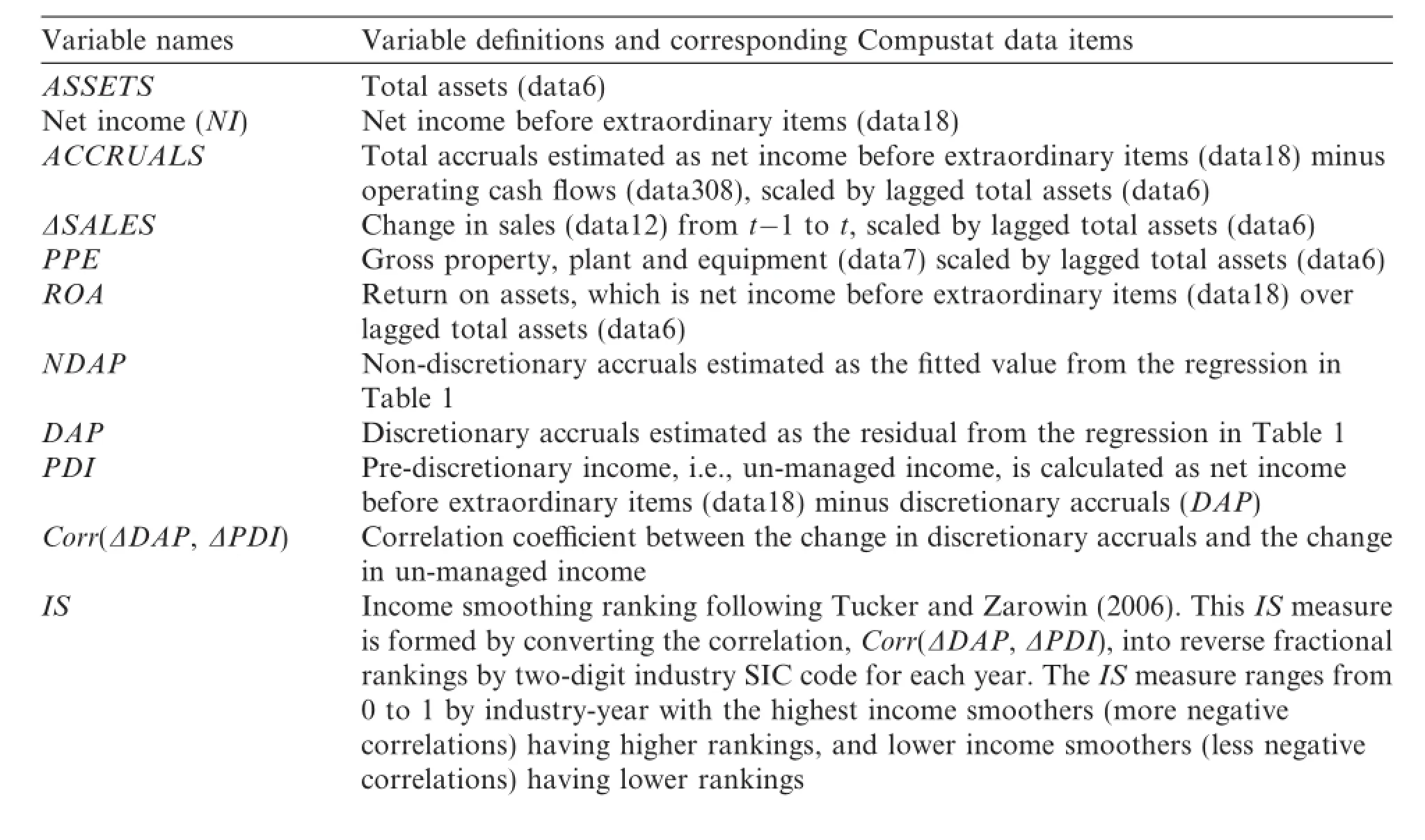
Variable namesVariable definitions and corresponding Compustat data items ASSETSTotal assets（data6）Net income（NI）Net income before extraordinary items（data18）ACCRUALSTotal accruals estimated as net income before extraordinary items（data18）minus operating cash flows（data308），scaled by lagged total assets（data6）ΔSALESChange in sales（data12）from t-1 to t，scaled by lagged total assets（data6）PPEGross property，plant and equipment（data7）scaled by lagged total assets（data6）ROAReturn on assets，which is net income before extraordinary items（data18）over lagged total assets（data6）NDAPNon-discretionary accruals estimated as the fitted value from the regression in Table 1 DAPDiscretionary accruals estimated as the residual from the regression in Table 1 PDIPre-discretionary income，i.e.，un-managed income，is calculated as net income before extraordinary items（data18）minus discretionary accruals（DAP）Corr（ΔDAP，ΔPDI）Correlation coefficient between the change in discretionary accruals and the change in un-managed income ISIncome smoothing ranking following Tucker and Zarowin（2006）.This IS measure is formed by converting the correlation，Corr（ΔDAP，ΔPDI），into reverse fractional rankings by two-digit industry SIC code for each year.The IS measure ranges from 0 to 1 by industry-year with the highest income smoothers（more negative correlations）having higher rankings，and lower income smoothers（less negative correlations）having lower rankings

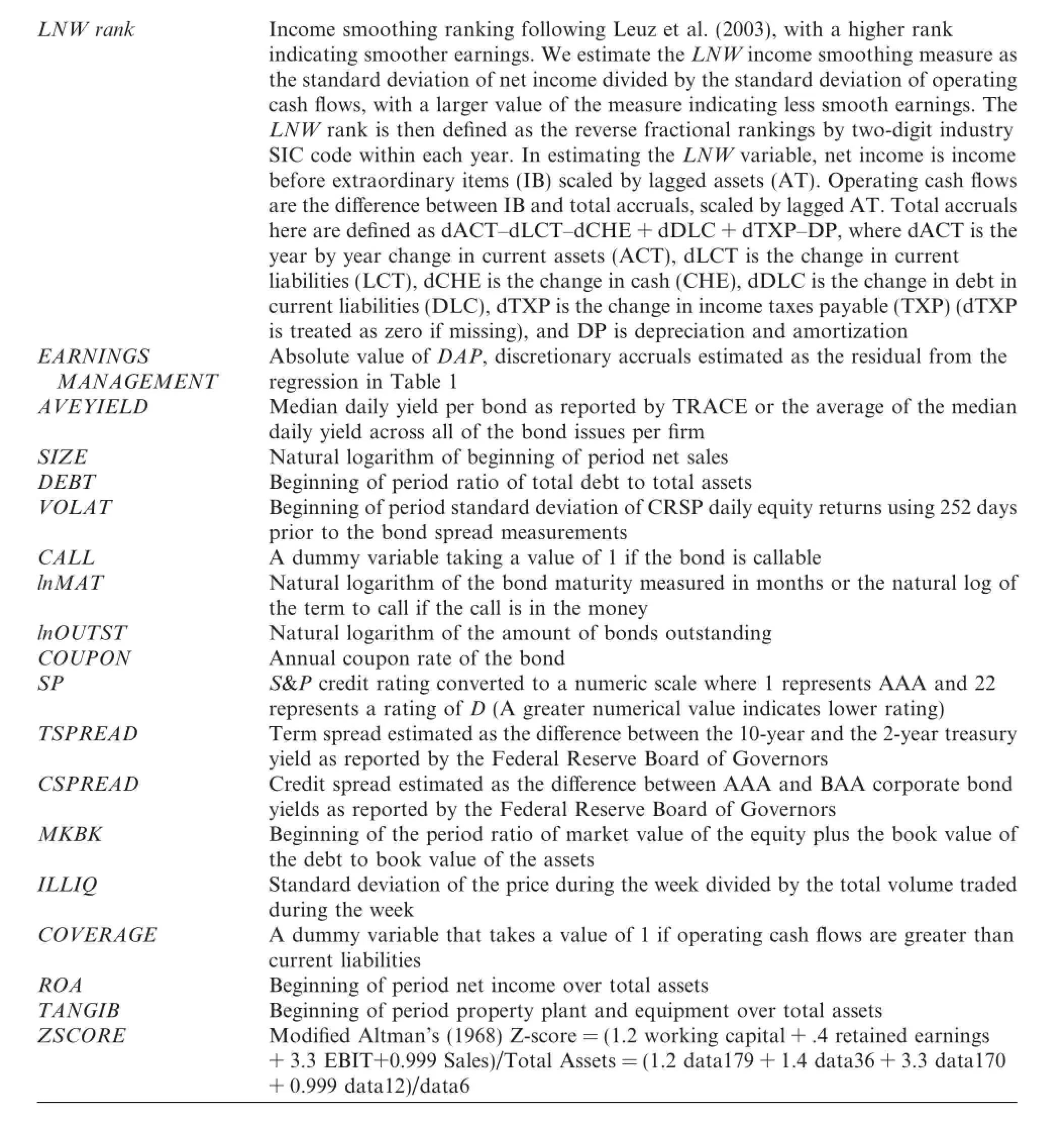
LNW rankIncome smoothing ranking following Leuz et al.（2003），with a higher rank indicating smoother earnings.We estimate the LNW income smoothing measure as the standard deviation of net income divided by the standard deviation of operating cash flows，with a larger value of the measure indicating less smooth earnings.The LNW rank is then defined as the reverse fractional rankings by two-digit industry SIC code within each year.In estimating the LNW variable，net income is income before extraordinary items（IB）scaled by lagged assets（AT）.Operating cash flows are the difference between IB and total accruals，scaled by lagged AT.Total accruals here are defined as dACT-dLCT-dCHE+dDLC+dTXP-DP，where dACT is the year by year change in current assets（ACT），dLCT is the change in current liabilities（LCT），dCHE is the change in cash（CHE），dDLC is the change in debt in current liabilities（DLC），dTXP is the change in income taxes payable（TXP）（dTXP is treated as zero if missing），and DP is depreciation and amortization EARNINGSAbsolute value of DAP，discretionary accruals estimated as the residual from the MANAGEMENTregression in Table 1 AVEYIELDMedian daily yield per bond as reported by TRACE or the average of the median daily yield across all of the bond issues per firm SIZENatural logarithm of beginning of period net sales DEBTBeginning of period ratio of total debt to total assets VOLATBeginning of period standard deviation of CRSP daily equity returns using 252 days prior to the bond spread measurements CALLA dummy variable taking a value of 1 if the bond is callable lnMATNatural logarithm of the bond maturity measured in months or the natural log of the term to call if the call is in the money lnOUTSTNatural logarithm of the amount of bonds outstanding COUPONAnnual coupon rate of the bond SPS&P credit rating converted to a numeric scale where 1 represents AAA and 22 represents a rating of D（A greater numerical value indicates lower rating）TSPREADTerm spread estimated as the difference between the 10-year and the 2-year treasury yield as reported by the Federal Reserve Board of Governors CSPREADCredit spread estimated as the difference between AAA and BAA corporate bond yields as reported by the Federal Reserve Board of Governors MKBKBeginning of the period ratio of market value of the equity plus the book value of the debt to book value of the assets ILLIQStandard deviation of the price during the week divided by the total volume traded during the week COVERAGEA dummy variable that takes a value of 1 if operating cash flows are greater than current liabilities ROABeginning of period net income over total assets TANGIBBeginning of period property plant and equipment over total assets ZSCOREModified Altman's（1968）Z-score=（1.2 working capital+.4 retained earnings +3.3 EBIT+0.999 Sales）/Total Assets=（1.2 data179+1.4 data36+3.3 data170 +0.999 data12）/data6

References

Aivazian，F.，Booth，L.，Cleary，S.，2006.Dividend smoothing and debt ratings.J.Financ.Quant.Anal.41（2），439-453.

Altman，E.，1968.Financial ratios，discriminant analysis and the prediction of corporate bankruptcy.J.Finance 23（4），589-609.

Arya，A.，Glover，J.，Sunder，S.，1998.Earnings management and the revelation principle.Rev.Acc.Stud.3，7-34.

Beidleman，C.，1973.Income smoothing:the role of management.Account.Rev.48（4），653-667.

Bessembinder，H.，Kahle，K.，Maxwell，W.，Xu，D.，2008.Measuring abnormal bond performance.University of Utah.（Unpublished working paper）.

Chen，N.，Roll，R.，Ross，S.，1986.Economic forces and the stock market.J.Bus.59（3），383-403.

Chen，L.，Lesmond，D.，Wei，J.，2007.Corporate yield spreads and bond liquidity.J.Finance 62（1），119-149.

Collin-Dufresne，P.，Goldstein，R.，Martin，J.，2001.The determinants of credit spread changes.J.Finance 56（6），2177-2207.

Dechow，P.，Hutton，A.，Sloan，R.，1995.Detecting earnings management.Account.Rev.70（2），193-225.

Demski，J.，1998.Performance measure manipulation.Contemp.Account.Res.15（3），261-285.

Demski，J.，Frimor，H.，1999.Performance measure garbling under renegotiation in multi-period agencies.J.Account.Res.37（Supplement），187-214.

Dichev，I.，Graham，J.，Harvey，C.，Rajgopal，S.，2013.Earnings quality:evidence from the field.J.Account.Econ.56，1-33.

Duffie，D.，Lando，D.，2001.Term structures of credit spreads with incomplete accounting information.Econometrica 69，633-664.

Edwards，A.，Harris，L.，Piwowar，M.，2007.Corporate bond market transaction costs and transparency.J.Finance 2，1421-1451.

Fama，E.，French，K.，1993.Common risk factors in the returns of stocks and bonds.J.Financ.Econ.33（1），3-56.

Fudenberg，D.，Tirole，J.，1995.A theory of income and dividend smoothing based on incumbency rents.J.Political Economy 103（1），75-93.

Goel，A.，2003.Why do firms smooth earnings？J.Bus.76，151-192.

Graham，J.，Harvey，C.，Rajgopal，S.，2005.The economic implications of corporate financial reporting.J.Account.Econ.40，3-75.

Healy，P.，1985.The effect of bonus schemes on accounting decisions.J.Account.Econ.20，125-153.

Hunt，A.，Moyer，S.，Shevlin，T.，2000.Earnings volatility，earnings management，and equity value.University of Washington.（Unpublished working paper）.

Jones，J.，1991.Earnings management during import relief investigations.J.Account.Res.29（2），193-228.

Kirschenheiter，M.，Melumad，N.，2002.Can big bath and earnings smoothing co-exist as equilibrium financial reporting strategies？J.Account.Res.40（3），761-796.

Kothari，S.，Leone，A.，Wasley，C.，2005.Performance matched discretionary accruals.J.Account.Econ.39（1），161-197.

Lambert，R.，1984.Income smoothing as rational equilibrium behavior.Account.Rev.41（4），604-618.

Lang，M.，Maffett，M.，2011.Economic effects of transparency in international equity markets:a review and suggestions for future research.Found.Trends Account.5，175-241.

Leuz，C.，Nanda，D.，Wysocki，P.，2003.Investor protection and earnings management.J.Financial Econ.69，505-527.

Miller，M.，Rock，K.，1985.Dividend policy under asymmetric information.J.Finance 40，1031-1051.

Myers，L.，Skinner，D.，2002.Earnings momentum and earnings management.University of Michigan.（Unpublished working paper）.

Ronen，J.，Sadan，S.，1981.Smoothing Income Numbers:Means，Objectives，and Implications.Addison-Wesley Publishing Company，Boston，MA.

Sankar，M.，Subramanyam，K.，2001.Reporting discretion and private information communication through earnings.J.Account.Res.39（2），365-386.

Srinidhi，B.，Ronen，J.，Maindiratta，A.，2001.Market imperfections as the cause of accounting income smoothing-the case of differential capital access.Rev.Quant.Financ.Acc.17，283-300.

Subramanyam，K.，1996.The pricing of discretionary accruals.J.Account.Econ.22，249-281.

Tang，D.，Yan，H.，2006.Liquidity and credit default swap spreads.Kennesaw State University.（Unpublished working paper）.

Trueman，B.，Titman，S.，1988.An explanation for accounting income smoothing.J.Account.Res.26，127-139.

Tucker，J.，Zarowin，P.，2006.Does income smoothing improve earnings informativeness.Account.Rev.81（1），251-270.

Verrecchia，R.，1983.Discretionary disclosure.J.Account.Econ.5，179-194.

Yu，F.，2005.Accounting transparency and the term structure of credit spreads.J.Financial Econ.75（1），53-84.

24 July 2015

.Tel.:+1 910 962 3606.

E-mail addresses:sli@wlu.ca（S.Li），Richien@uncw.edu（N.Richie）.1Tel.:+1 519 884 0710x2395.