A direct probabilistic approach to solve state equations for nonlinear systems under random excitation

Zheng Lv·Zhiping Qiu



RESEARCH PAPER

A direct probabilistic approach to solve state equations for nonlinear systems under random excitation

Zheng Lv1·Zhiping Qiu1

In this paper，a direct probabilistic approach（DPA）is presented to formulate and solve momentequations for nonlinear systems excited by environmental loads that can be either a stationary or nonstationary random process. The proposed method has the advantage of obtaining the response’s moments directly from the initial conditions and statistical characteristics of the corresponding external excitations.First，the response’s moment equations are directly derived based on a DPA，which is completely independent of the Itô/filtering approach since no specific assumptions regarding the correlation structure of excitation are made. By solving them under Gaussian closure，the response’s moments can be obtained.Subsequently，a multiscale algorithm for the numerical solution of moment equations is exploited to improve computational efficiency and avoid much wall-clock time.Finally，a comparison of the results with Monte Carlo（MC）simulation gives good agreement. Furthermore，the advantage of the multiscale algorithm in terms of efficiency is also demonstrated by an engineering example.

Direct probabilistic approach·Nonlinear dynamic system·Nonstationary random process· Response’s moments·Multiscale algorithm

✉ Zheng Lv lvbaolvzheng@126.com

1Institute of Solid Mechanics，Beihang University，Beijing 100191，China

1　Introduction

Earthquakes，wind，and wind waves in the sea represent common environmental loads.Artificial structures can be excited by environmental loads，for example，building on land exhibiting dynamic responses affect their functionality and safety［1］.In many engineering problems，dynamic theory has mainly dealt with structures with deterministic parameters and external loads.However，the parameters of such problems contain uncertainties，for example，material properties，structural geometry，and the external loads.In particular，the uncertainties in the external loads are more serious.Therefore，it is more appropriate for engineers to solve engineering problems using an uncertainty analysis method.

Of the numerous uncertainty analysis methods，such as probabilistic and statistical models［2-5］，nonprobabilistic convex models［6-8］，fuzzy mathematics［9］，and interval analysis［10］descriptions，the probabilistic method is the most important for researchers and engineers because it produces well-defined results for specified levels of reliability.To study the response of a dynamical system，we must formulate and solve stochastic differential equations. Based on current studies in the literature that present structural response problems with random uncertainties，there are fourmain methods:Monte Carlo（MC）simulation，statistical linearization，Fokker-Planck-Kolmogorov（FPK）equation，and the moment equation approach.

The MCapproach isconceptually［11-13］straightforward and has the advantage of being applicable to both linear and nonlinear structural random response analysis，but it is computationally costly.The FPK equation is essentially equivalent to the Itô stochastic differential equation，which iswidely used in the analysis ofnonlineardynamicalsystemsunderdelta-correlated excitation［14］.However，in the case of smoothly correlated excitation，the FPKapproach isavailable only under the assumption that excitation can be represented by the output of an appropriate filter excited by white noise［15-18］.Although the range of applicability of the FPK approach has been extended using a stochastic averaging approach and a filtering approach，ithas two drawbacks:first，it restricts random excitation to delta-correlated processes or processes that can be modeled as the output of a stochastic filter；second，itincreases the numberofstates ofthe moment system to be solved.Thus，many researchers have paid more attention to some statistical moments and tried to formulate and solve moment equations.For example，Lutes and Papadimitriou［14］investigated the response of a nonlinear system subjected to a delta-correlated process and proposed a relatively straightforward formulation for deriving the differential equations of the response moments and cumulants of a dynamical system.Di Paola and Floris［17］focused on the statistical characterization of the non-Gaussian response of nonlinear systems excited by polynomial forms of filtered Gaussian processes.As noted earlier，much effort has been devoted to analyzing the statistical moments of the response of a dynamical system.However，most theoretical studies ignore the improvement in efficiency from the numerical algorithm.Obviously，this may lead to some difficulties in practical applications，especially for large-scale engineering problems.In addition，delta-correlated excitation is often used to formulate moment equations，but such excitation is not valid in the case of environmental loads.In fact，Qiu and Wu［19］have investigated dynamicalsystems excited by environmental loads and pointed out that the direct probabilistic approach is very efficient at solving state equations under random excitation.However，their research is limited to linear problems.

In this paper，we propose a direct probabilistic approach（DPA）to formulating and solving momentequations fornonlinear systems excited by environmental loads.At the same time，a novel multiscale algorithm for the proposed method is exploited.In the proposed method，the derivation of the momentequations is completely independentofthe classical method using the FPK/Itô/filtering approach.The statistical moments of the response can be directly obtained from the initial condition and the statistical characteristics of the corresponding external excitations.Furthermore，the multiscale algorithm can be used to improve computational efficiency in large-scale practical engineering problems.

The remainder of this paper is organized into seven sections as follows.In the nextsection，the problem formulation is discussed.Then Sect.3 presents the DPA to formulating moment equations of nonlinear systems.We obtain closed momentequations undersome assumptions in Sect.4.Based on the proposed method，in Sect.5，a multiscale algorithm is designed to numerically solve moment equations.The numerical results are presented in Sect.6.Finally，conclusions are drawn in Sect.7.

2　Problem statement and notation

The general form of a differential equation for a nonlinear system with n degrees of freedom（DOFs）can be given by

where M，f，and Q are the generalized mass matrix，nonlinear function，and external load vector，respectively.y，˙y，and¨y are the generalized displacement，velocity and acceleration vectors，respectively.

In thispaper，we focus on the simplestcase ofa differential equation with cubic nonlinearity under random excitation. Equation（1）can be written as

where the◦sign is the Hadamard product，which represents the corresponding terms in two vectors multiplied，and the result is still a vector.

The dynamic system associated with Eq.（2）can be reduced to standard form by introducing the 2n-dimensional state vector and the 2n-dimensional excitation vector

Then Eq.（2）can be written in the form

where the matrices A1，A3，and B are both 2n×2ndimensional and real

Itis noteworthy thatthe first n equations in the state-space equation represent the equations of motion given by Eq.（2），and the other n represent the identities

Forconvenience we use the following notation throughout the paper.For the sake of generality，the notation

will be used to express the joint moment of order j1+j2for any two random functions x（t），y（τ）.

The preceding notation is unambiguous except in the case x=y，t=τ，where the moment function can be written in various equivalent forms.Allcouples（j1，j2）with j1+j2= j representthe same j-th-ordermomentof x（t）.Forexample，

Similarnotation is also used forthe jointmomentofthe three random functions

3　Direct probabilistic approach

In thissection，using the DPA，we willderive the matrix equations of the moment of interest under no approximations or assumptions except for the assumed existence of the various mathematically expected values.

3.1Moment equations for mean of dynamic responses

Consider the external excitations of a dynamical system of structurescontaining randomuncertainties.Adynamicalsystem of structures with cubic nonlinearity may be described in general by the 2n-dimensional state-space equation

where x（t）is the 2n-dimensional state-space variable vector，A1and A3are the 2n×2n-dimensional system matrix，B is the 2n×2n-dimensional input matrix，and u（t）is the 2ndimensional input vector.In this paper，the matrices A1，A3，and B are deterministic，and the vector u（t）denotesa random process.Therefore，the state-space variable vector x（t）isalso a random process.

By taking the mathematical expectation of Eq.（8），the mean or first-order moment equations can be obtained as follows

Using the expression

and considering the notation in Sect.2，Eq.（9）can be rewritten as

Using the DPA，the average state equation for a nonlinear system under random excitation is derived.It can be seen from Eq.（11）thatthe third-orderresponse moment Rx◦x◦x（t）ispresentowing to the existence ofa cubic nonlinearity term. Obviously，the mean vector mx（t）of the dynamic response vector x（t）cannot be directly obtained from Eq.（11）even if the initial condition and the excitation’s mean value are known.

3.2Moment equations for correlation matrix

To obtain the correlation matrix of the dynamic responses of structures with uncertainties，the matrix x（t）xT（τ）of the state-space variable must be constructed based on the 2ndimensional state-space equation of a dynamical system of structures with cubic nonlinearity.To do this，both sides of Eq.（8），being multiplied by the stochastic vector xT（τ），give

Taking the mathematical expectation of Eq.（12）and considering Eq.（10），we obtain the correlation matrix equations

Equation（13）is a set of first-order partial differential equation，and the initial condition Rxx（t0，τ）and the input of the equation Rux（t，τ）are needed to obtain the solution.

Setting the time variable t=τ and taking a transposition of Eq.（8），we get

and Eq.（14），being a left multiplication by x（t0），gives

In a similar manner，the following equation is obtained

Equation（16）is a setoffirst-orderordinary differentialequation，and in this paper，the initial condition Rxx（t0，τ0）and the input of the equation Rxu（t0，τ）are known.

Equation（14），being a left multiplication by u（t），gives

In a similar manner，the following equation is obtained

where the inputitem Ruu（t，τ）isthe correlation matrix ofthe externalrandomexcitation，which in this paperis known，and the Rux（t，τ0）is also known.

3.3Moment equations for covariance matrix

Two methods can be used to obtain the covariance matrix of the response.In the first one，if the mean and correlation matrix were already obtained in Sect.3，then the covariance matrix can be obtained by the relationship between the covariance matrices and correlation matrices，

In addition，an equation for the covariance matrix can be obtained using an approach similar to that used to obtain Eq.（13）.

Subtracting Eq.（11）from Eq.（8）yields the following equation

Both sides of Eq.（20），being multiplied by Eq.（21），give

Considering the independence between the arguments t and τ，and taking the mathematical expectation of Eq.（22），the covariance matrix equations can be obtained as follows

Expanding the third term in Eq.（23），we obtain

Substituting Eq.（24）in Eq.（23），Eq.（23）simplifies to

Aswith solving the sequence ofEq.（13），to solve Eq.（25）we also need the input item Cux（t，τ）and the initial condition

Cxx（t0，τ）.Forconvenience and to save space，the first-order ordinary differential equations for Cxx（t0，τ）and the firstorder partial differential equations for Cux（t，τ）are directly given as

3.4Moment equations for mean square function and variance function

According to the definition of the mean square function and the derivation rule，we obtain

Let the time variable τ in Eq.（12）be t；substituting Eq.（12）and transposing Eq.（12）into Eq.（28），Eq.（28）can be written as

By taking the mathematicalexpectation ofEq.（29），the mean square function equation can be obtained

Following the foregoing procedure for Eq.（30），the crosscorrelation functions with the same argument t，Rux（t，t）and Rxu（t，t）can be obtained by solving the following equations

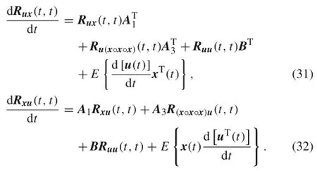
It can be seen from Eqs.（31）and（32）that in this paper， the initial conditionand the variance function ofthe externalrandom excitation Ruu（t，t）are known.

Following the foregoing procedure for Eq.（30），we can also obtain the moment equation for the variance function as follows

The preceding equation is very complicated compared to Eq.（25）.It is inconvenient to solve Eq.（33）for the variance function，so we will introduce a simple method to obtain the variance function.

As it is commonly known，the relationship between the mean square function and the variance function is

Itcan be clearly seen from Eq.（34）thatthe variance function can be readily obtained when the mean square function is known.In fact，Eq.（33）is not closed and can be solved only after we calculate the solution of the mean square function of the response，which is obviously different from that of linear systems.Therefore，under the premise of the known mean square function，Eq.（34）is more easily solved for the variance function than Eq.（33）.

Up to this point，the matrix equations of a response’s statistical moments have been derived based on the DPA.In the case of linear systems，it is straightforward to obtain closed momentequations，see forexample，the research published by Qiu and Wu［19］.For nonlinear systems，however，the formulation of moment equations involves higher-order moments owing to the existence of cubic nonlinearity terms. Obviously，the matrix equations ofthe momentobtained earlier are not closed.In the section that follows，we describe how to solve moment equations for a response’s statistical moments.Itis noteworthy thatno approximations orassumptions are made in deriving the moment equations，other than the assumed existence of the various mathematically expected values；therefore，the obtained moment equations are exact in this paper.

4　Closed moment equations for mean，correlation，and mean square function of response

To eliminate higher-order moments from the nonclosed moment equations derived in Sect.3，one must adopt a suitable closure approximation，such as the hypothesis of normality or quasi-normality of the dynamic response.In this section，the simplest case to consider is to accept the hypothesis of normality of the dynamic response，the socalled Gaussian closure.In this case，all cumulants of order greater than two are equal to zero.By virtue of the definition and the formulas ofcumulantexpansion，closed moment equations for the response’s statistical moments are to be given.

For the sake of simplicity，we will first introduce the closure technique for a single-degree-of-freedom nonlinear state-space equation.The extension to multidegree-offreedom nonlineardynamicalsystems is straightforward.Let the degree of freedom be one；Eq.（8），the state-space equation，can be written

Similarly，the nonclosed moment equations derived from the state-space equation by the DPAare directly given as follows

To apply Gaussian closure，we need to build the relationship between the cumulant and moment of random variables by using the characteristic function of normality.In elementary probability theory，the cumulants of the first-and second-order are equal to the mathematical expectation and covariance of random variables，respectively.The relation formula between the cumulant and moment ofthree and four random variables can be expressed in the following form:

where κpis the p-th-order cumulant of a random variable. Under the Gaussian closure assumption，all cumulants of order greater than two are equal to zero.Thus，we have

Note that the fourth-order moment is further related by certain expressions to moments of the first-and second-order.If the random variables are modeled as zero-mean uncorrelated Gaussian random variables，then all the central moments of an odd order（starting from the third）turn out to be equal to zero，and moments of an even order are related by certain expressions to moments of the second-order.

Applying the preceding equations to Eqs.（36）-（39），the closed moment equations can be obtained as follows

It can be seen from Eqs.（42）-（45）that the closed moment equationsinvolve an unknown term，which isthe mean square function of the response.Thus，to solve the closed moment equations，it is necessary to add the closed moment equations of the mean square function of the response.Applying Eq.（41）to Eqs.（30）and（31），we obtain

When the solutions for moments mx（t），Rxx（t，t），and Rxx（t，τ）are obtained from Eqs.（42）-（47），it is very convenient to calculate the correlation moments Cxx（t，τ）and Cxx（t，t）from Eqs.（19）and（34），respectively.

So far，the closed moment equations for mean，correlation，and mean square functions of the response have been obtained under a Gaussian closure assumption.We are able to solve the system of equations for the response’s moment. In fact，the Gaussian closure assumption is equivalent to the second-order cumulant neglect closure assumption.In addition，the closed moment equations can be obtained under another assumption.It is noteworthy that the correlation matrix can be obtained only after we have calculated the solution of the mean square function of the response，which is also obviously different from that of linear systems.

5　Multiscale algorithm of moment equations

Although the statistical moments of the response can be directly obtained from the initial condition and the statistical characteristics of the corresponding external excitations，it can be seen thatwe mustsolve a differential equation system consisting of Eqs.（42）-（47）.For large-scale practical engineering problems，the runtime and the computations are verylarge.To overcome the disadvantages of the large number of calculations，in this section，we introduce a multiscale algorithm of the moment equations，which can be quite suitable for large-scale computations to avoid excessive wall-clock time.

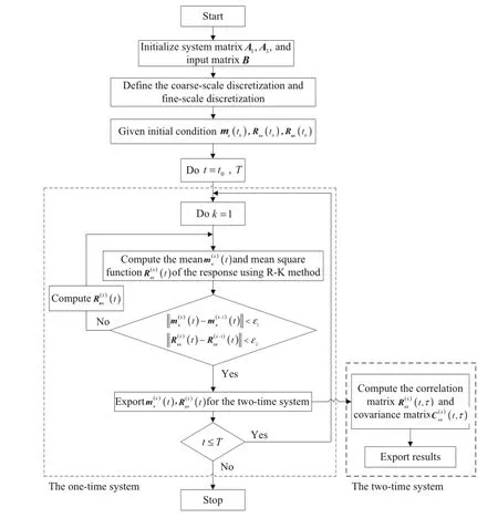
Fig.1 Flowchart of multiscale arithmetic

Aflowchartofthe multiscale algorithm isshown in Fig.1. The solution scheme will be defined in the time interval［t0，T］，which is considered to be a long time enough for the system to reach the long-time statistical equilibrium limit.This time interval is discretized by a discretization D coarse=｛ti:t0=t0＜t1＜···＜tI=T｝，and each of its subintervals[ti，ti+1]is further discretized by intermediate time points ti，j，j=0，1，···，Ji，forming the fine-scale discretizationOwing to the existence of two-time variables t and τ， the closed moment equations can be naturally split into two systems，the one-time system of Eqs.（42），（46），and（47），and the two-time system of Eqs.（43）-（45）.For the one-time system，the solution procedure is initialized using the initial condition mx（t0），Rxx（t0），and Rux（t0）.The mean and mean square function of the response can be solved numerically in the first time interval［t0，t1］of the coarse-scale discretization，namely，the fine-scale discretizationIn the first cycle of the iterative procedure（k=1），the unknown cross correlation Rux（t，t）isassumed to remain constantand equal to its initial values.Under this assumption，the one-time sys-tem of equations can be rewritten in the following form

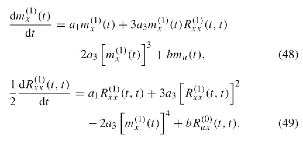
The first-cycle iteration of the scheme is completed following calculation of the solution to Eq.（50）.In the second cycle ofthe iterative procedure（k=2），the cross correlation）is used to calculate the quantitiesinstead of

Following the foregoing procedure forcan be obtained in the fine-scale discretizationsimultaneously，can be.The iterative procedure continues to higher-order cycles in the same way until the following convergent conditions are met

As shown in Fig.1，the numerical scheme can advance to the second time interval［t1，t2］of the coarse-scale discretization when the convergence conditions are met.It is noteworthy that，to accelerate the convergence，the initial condition can be obtained by linearly extrapolating the last two available values from the previous coarse-scale time interval.

For the two-time system，it is very convenient to calculate the correlation moment after having calculated the solution of the one-time system.Because mx（t）and Rxx（t，t）are known，Eqs.（44）and（45）are typical linear ordinary differential equations with respect to the response time τ.The solutions of Eqs.（44）and（45）are the initial condition and coefficient of Eq.（43），respectively.Obviously，the correlation moment of the response can be obtained by solving Eq.（43），which is a standard ordinary differential equation with respect to the response time t，and be parametrically dependent on the second time τ.

For a conventional algorithm，it is necessary to solve a differentialequation systemconsisting of Eqs.（42），（46），and（47）at the same time.However，in this algorithm，we need to only solve the differential equation system consisting of Eqs.（42）and（46），and then Eq.（47）is solved.Therefore，the calculation time using the multiscale algorithm is less than that of the conventional algorithm if the same precision is required.

6　Numerical examples

The implementation of the DPA is illustrated using three examples in this section.Two numerical examples，a singledegree-of-freedom oscillator and a multistory shear building structure，are presented to show the good performance of the proposed method in a nonlinear system，and the last one，a multistage power pagoda，is used for an engineering application of the proposed method.Meanwhile，the advantage of the multiscale algorithmin terms ofefficiency isalso demonstrated.

6.1Response of a single-degree-of-freedom oscillator to random excitation

Consider a single-degree-of-freedom oscillator subjected to a horizontal acceleration at the base shown in Fig.2 and described by the differential equation

It is assumed that the generalized mass matrix，damping matrix，and stiffness matrix are deterministic parameters，and their numbers are M=10 kg，C=2000 N·s/m，and

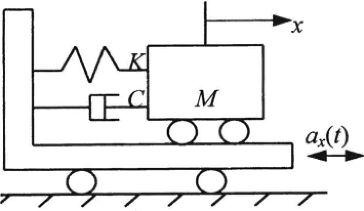
Fig.2 System model

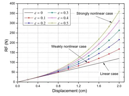
Fig.3 RF for various intensities of nonlinearity

K=6 kN/m，respectively.The mean value and standard variance of the random parameter θ are μθ=20 cm/s2and σθ=5.

To expose the intensity of the system nonlinearity clearly，the restoring force（RF）ofthe systemiscalculated forvarious intensities of nonlinearity，as shown in Fig.3，in which the displacement considered ranges from 0 to 2 cm.From Fig.3 it is observed that for very low values of displacement，the nonlineareffectofthe RFis notobvious.With the increase in displacements，a clear deviation is shown from the linear RF. For a clear comparison，Table 1 lists the amplification factor（AF）of the linear RF at different displacements.The data in Table 1 indicate that the AF of the linear RF ranges from 1.144 to 1.4 for ε=0.1，while that of ε=0.5 ranges from 1.72 to 3，which clearly reveals the intensity of the system nonlinearity.Furthermore，the mean values of the RF，speed，and displacement response for various intensities of nonlinearity are plotted in Fig.4.According to the comparison of the responses in the figure，a strongernonlinearity results in a smaller value of the response’s statistical moments，which is expected owing to the fact that the restoring effect of the linear term is amplified because the coefficient of the nonlinear term in the state equation is negative.

For verification purposes，numerical results for the mean and variance of the response are，respectively，solved via the proposed DPA and MC simulation plotted in Figs.5-8.The coefficient of the nonlinear term ε is taken as ε=0，0.1，and 0.5（linear，weakly/strongly nonlinearcase，respectively）.For each case，an MC simulation with a sample size of 10000 is used to generate the reference results，which we take to represent the“true”values for the response.

Figure 5a and 5b shows the mean values of speed and displacement response，respectively，in which the red curve is the solution of the MC simulation and the blue point is the solution of the proposed DPA，and Fig.6 shows the variance ofthe response.We can see thatfora linearsystem the results from the DPA are in excellent agreement with the MC simulation.The good performance ofthe proposed method can be attributed to the fact that no approximations or assumptions were made in the linear system.

Figure 7a and 7c shows the mean values of the speed and displacement response for a weakly nonlinear system，respectively.It can be seen clearly that the performance of the proposed method is very good in the nonlinear case as well，even though nonlinearity leads to small values of the response’sstatisticalmoments.Furthermore，we can see from Fig.8 that for the strongly nonlinear case，the difference in the results using the two methods becomes noticeable owing to the inaccuracy caused by the Gaussian closure assumption.

As shown in Figs.5-8，the relative error of the DPA increases gradually with increases in ε，that is to say，a stronger nonlinearity leads to a larger relative error.However，we must recognize that the simplest moment closure is the fundamentalcause ofthe errorofthe response’sstatistical moments in this paper.Fora strongly nonlinearsystem，some types of advanced，non-Gaussian moment closure schemes can be applied to improve the accuracy of the DPA，such as cumulant-neglect closure，quasi-moment neglect closure，and polynomial-Gaussian closure.

Figure 9a and 9b shows the covariance of speed and displacementresponse aboutdifferenttime variables t andτ for a strongly nonlinearsystem，respectively，in which the covariance of speed and displacement response have a symmetric relationship about t=τ.Let the time variable t=τ；then we can get the variance of speed and displacement response from Fig.9a and 9b，which are shown in Fig.8b and 8d，respectively.

Table 1 AF of linear RF at different displacements

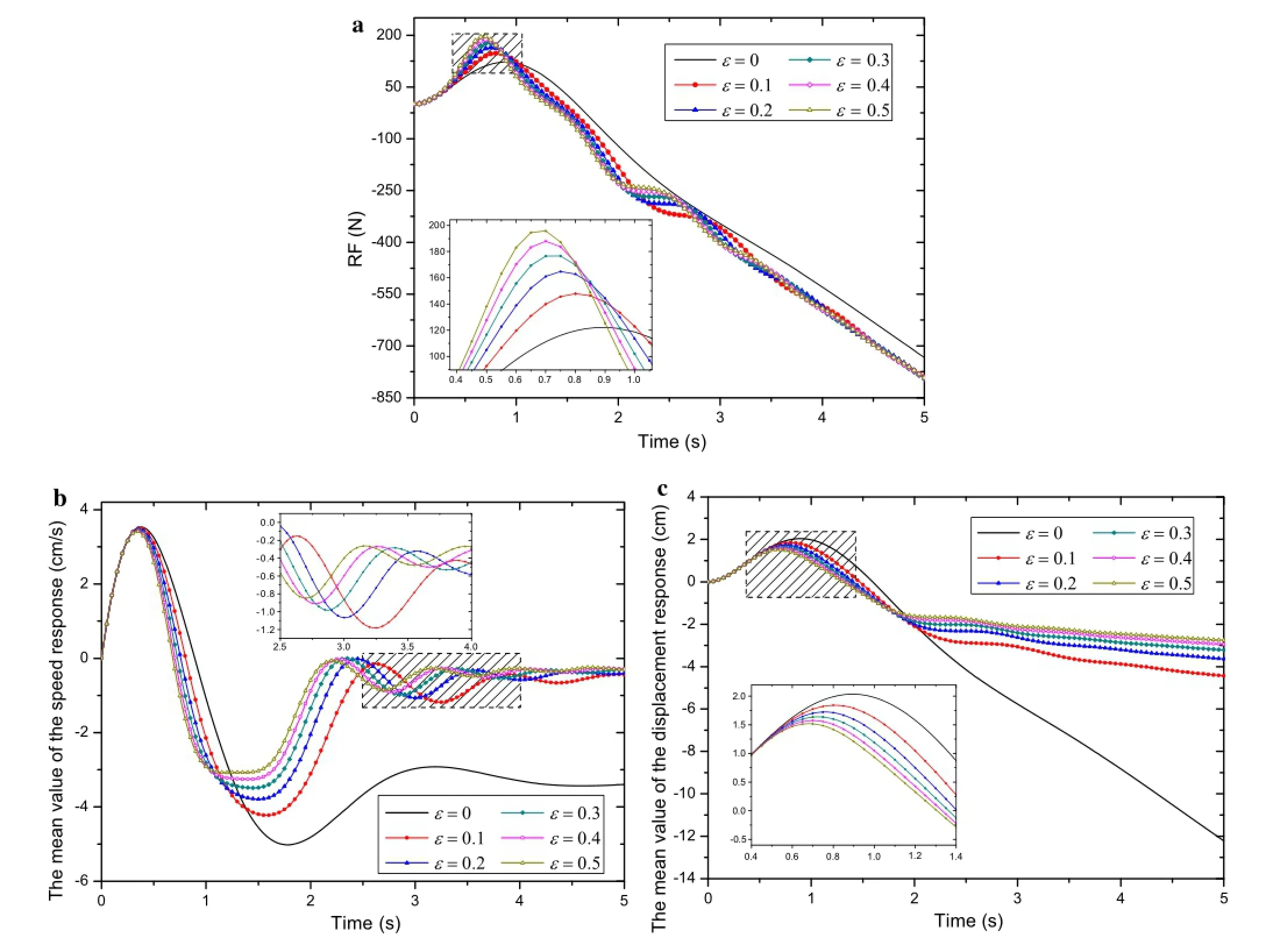
Fig.4（Color online）Mean value of response for various intensities of nonlinearity.a RF response.b Speed response.c Displacement response

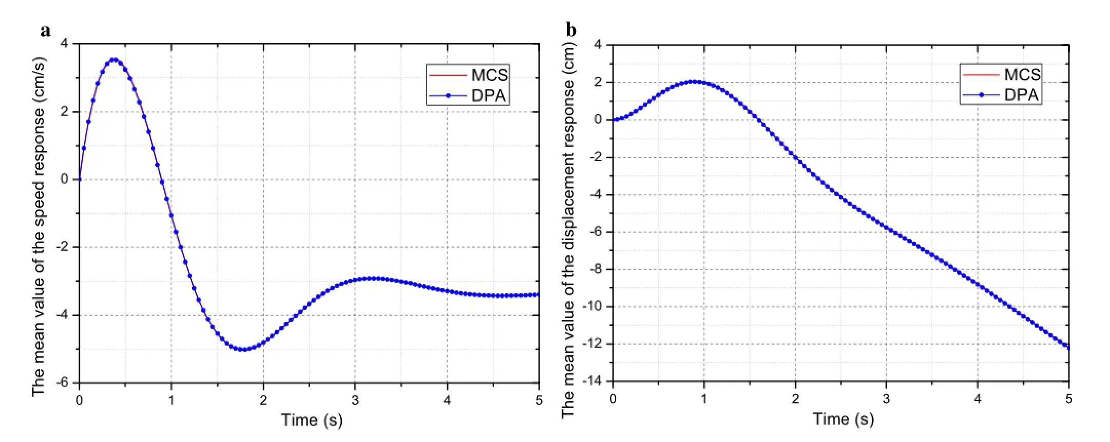
Fig.5（Color online）Mean value of response for linear system.a Speed response.b Displacement response

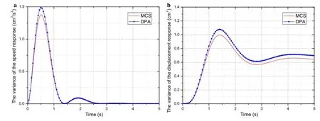
Fig.6（Color online）Variance of response for linear system.a Speed response.b Displacement response

Fig.7（Color online）Mean value of response for nonlinear system.a Speed response（ε=0.1）.b Speed response（ε=0.5）.c Displacement response（ε=0.1）.d Displacement response（ε=0.5）

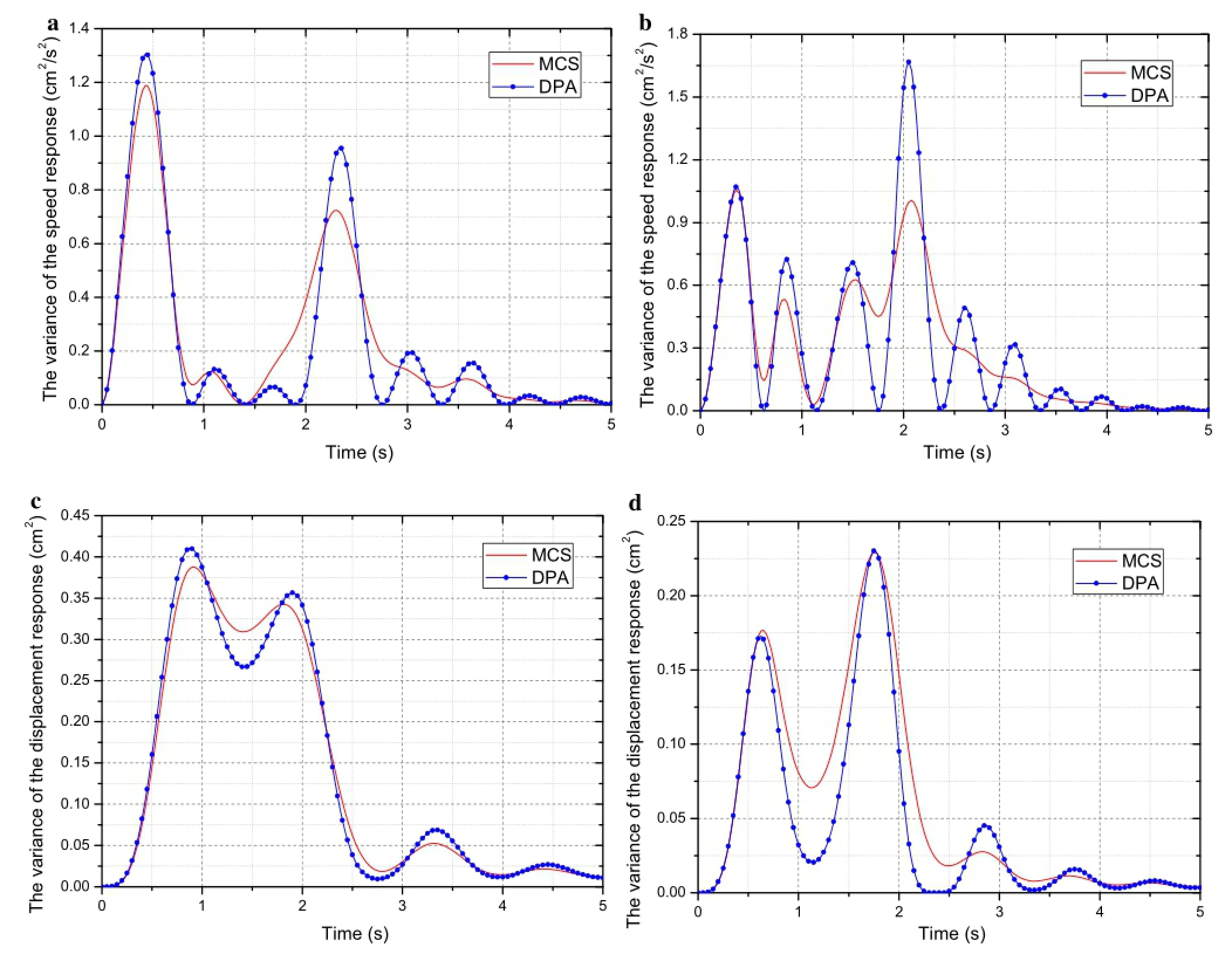
Fig.8（Coloronline）Variance of response fornonlinearsystem.a Speed response（ε=0.1）.b Speed response（ε=0.5）.c Displacementresponse（ε=0.1）.d Displacement response（ε=0.5）

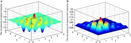
Fig.9（Color online）Covariance of response for strongly nonlinear system.a Speed response（ε=0.5）.b Displacement response（ε=0.5）

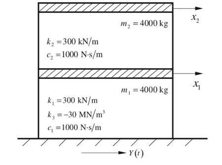
Fig.10 Double-story shear building structure

6.2Response of a multistory shear building structure to random earthquake-type disturbance

The previous example was presented to illustrate the accuracy and implementation of the proposed method.Next，we consider a double-story shear frame building structure with nonlinearstiffness（Fig.10）.The nonlineardifferentialequation is represented as

The structural parameters are marked in Fig.10.The following nonstationary random model will be used to simulate the ground acceleration caused by a strong earthquake

where the parameters aj，αj，ωj，and θjare assumed to be random variables and follow uniform distributions:aj～U（1，5），αj～U（0.5，1.5），ωj～U（10，50），θj～U（0，2π），respectively.In this example we let n=10，and a typical sample function of Y（t）is shown in Fig.11.

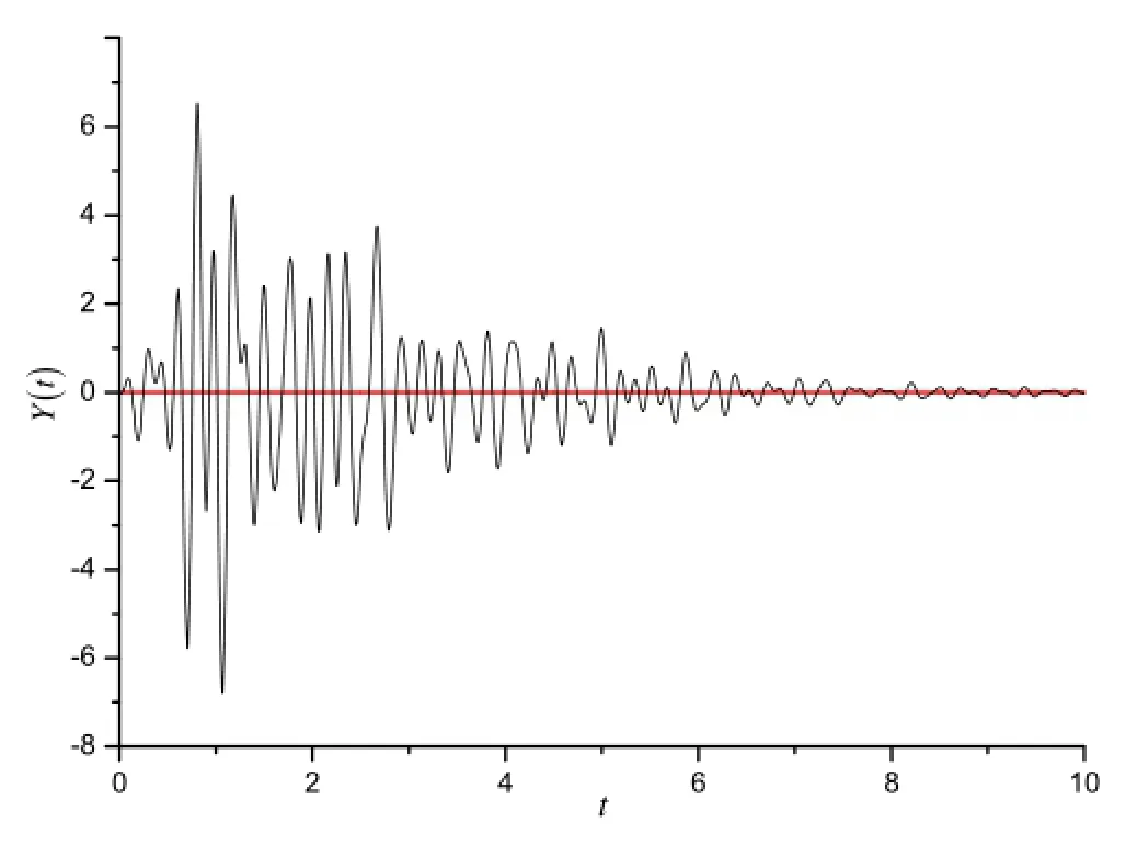
Fig.11 Typical sample function of ground acceleration excitation

The moment equations obtained based on the proposed method are solved for the response’s statistical moments. Meanwhile，MCsimulation isalso performed，and the results obtained by the proposed DPAare compared to those ofa MC simulation for verification purposes，where the sample size remains 10000.The mean values of the speed and displacement response are shown in Figs.12 and 13，respectively. As expected，the DPA gives good results that are mainly in agreement with the MC simulation，which indicates that the proposed method is appropriate forthe analysisofdynamical systems excited by environmentalloads such as earthquakes，wind，and wind wavesin the sea.Additionally，the covariance of the speed and displacement response is shown in Fig.14. We can see thatthe covariance ofthe speed and displacement response have a symmetric relationship about t=τ themselves.Figure 15 shows the cross covariance ofthe response，in which the symmetric relationship does not exist.All this is in accordance with the actual physical meaning.

In fact，because of insufficient data，it is very difficult to obtain the exact joint probability density functions.The available data may only be sufficient to estimate the first few statistical moments，such as the mean，variance，and correlations.The method proposed in this paper is more convenient for obtaining the moment of response from the initial conditions and the statistical characteristics of the corresponding external excitations.

6.3Response of multistage power pagoda with nonlinear stiffness

To demonstrate the advantage of the multiscale algorithm in terms of efficiency，a multistage power pagoda（Fig.16）is considered.In the figure，the structure is supported by just four columns with a rectangular cross section W120 mm× 120 mm×4 mm，and each stage is composed of pipes with a circular cross section Φ50 mm×5 mm.The Young’s modulus of the material is 2.06×105MPa.There is a harmonic sinusoidal excitation F（t）=-p sin（4πt）acting on the verticaldirection ofthe tip ofthe cantilever.The mean value and standard variance of random parameter p are μp=1960 N and σp=100，respectively.Suppose that the stiffness of the system is nonlinearand the nonlineardifferentialequation of the system can be represented as

Fig.12（Color online）Mean values of speed response.a Speed responseb Speed response

Fig.13（Color online）Mean values of displacement response.a Displacement response x1.b Displacement response x2

Fig.14　（Color online）Covariance of speed and displacement response.a Speed responseb Displacement response

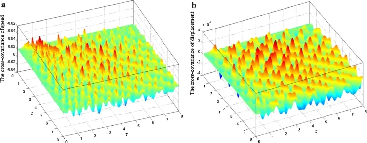
Fig.15（Color online）Cross covariance of speed and displacement response.a Speed responseb Displacement response C x1x2（t，τ）

Fig.16 Multistage power pagoda structure

where M and K are the linear mass matrix and stiffness matrix，respectively，and F（t）is the external force vector.

According to the DPA and its multiscale algorithm，an Finite Element Analysis（FEA）program coupled with existing deterministic finite-element（FE）codes is designed using MATLAB.In this program，a geometricalmodelofthe structure and mesh are created with the deterministic FE codes.In this example，the linear mass matrix and stiffness matrix are generated using Direct Matrix Abstraction Programming of MSC/Nastran，and a prediction of the response’s statisticalmoments for a nonlinear system is carried out in MATLAB R2012 on a 3.40 GHz Intel Core i7 4-CPU computer.

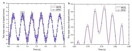
Fig.17（Color online）Mean values of speed response at tip of cantilever.a Speed responseb Amplification drawing

Fig.18（Color online）Mean values of displacement response at tip of cantilever.a Displacement response u3y.b Amplification drawing

Using the program，we obtain the dynamic response ofthe multistage power pagoda under random excitation.Because of space limitations，we only plot the mean values of the speed and displacement response at the tip of the cantilever（Figs.17 and 18，respectively）.The comparison in Figs.17 and 18 suggests thatthe proposed method yields good results for practical engineering problems.

For further investigation of the computational efficiency of the multiscale algorithm，a series of power pagoda problems with an increasing number of elements is considered. The number of elements for five power pagodas ranges from 488 to 920，while the number of DOFs ranges from 1500 to 2844.In some sense，the problems considered here are“large”scale.In this example，the timestep length is taken as △t=0.05 s，0.0125 s（coarse-scale and fine-scale，respectively）.Meanwhile，we also solve the moment equations using a conventional algorithm for the sake of comparison.

Table 2 summarizes the problem scale and the computation time of each problem solved by the multiscale and conventional algorithms.It is observed that with the increase in the problem scale，the computation time of conventional algorithm ranges from 510.544s to 633.114 s，while that of the multiscale algorithm ranges from 409.021 s to 487.245 s. As compared with the conventionalalgorithm，the multiscale algorithm spends much less time on all problems.

Additional useful information listed in Table 2 is the ratio of the computation time of the proposed algorithm to that of the conventional algorithm.This table suggests that the ratio is around 76%to 80%，which indicates the multiscale algorithm is superior to the conventional algorithm，and the time savings，especially forlarge-scale engineering problems，can be significant.Based on the data listed in Table 2，the com-

Table 2 Problem scale and computation time of two algorithms

Fig.19 Computation time versus problem scale

putation time of the two algorithms are plotted as functions of the number of DOFs（Fig.19）.

7　Conclusions

In this paper，a DPA is presented to formulate and solve moment equations for nonlinear systems under random excitation，which is completely independent of the classical method using the Itô/filtering approach.The proposed method allows us to deal with nonlinear systems under smoothly correlated excitations and has its own advantage of obtaining the statistical moments of a response directly from the initial conditions and the statistical characteristics of the corresponding external excitations.

Using three examples，numerical studies are presented to illustrate the implementation of the proposed method.The results computed using the DPA are compared with the reference results generated using a MC simulation.Based on the numerical studies，we conclude that the performance of the proposed method is very good in the nonlinear case，even though nonlinearity results in small values of the response’s statistical moments.Furthermore，it can be seen that the difference in the results in the strongly nonlinear case is greater than that in the weakly nonlinear case.The difference is attributed to the inaccuracy caused by the Gaussian closure assumption.Meanwhile，a multiscale algorithm is used to solve the moment equations and is shown to be superior to the conventionalalgorithm and improves computationalefficiency.Therefore，the multiscale algorithm can be used to solve large-scale engineering problems.

A weak point of this paper is that the whole analysis is based on the simplest moment closure，the Gaussian closure. For a strongly nonlinear system，the truncation error induced bythe Gaussian closure can be magnified andhasa significant effect on the dynamic response.Further work is required to apply modern non-Gaussian closure schemes to solve the moment equations to improve the accuracy of the proposed method.

A preliminary numerical study of DPA for static and dynamic problems of a linear system［19，20］has been published.This paperaimsto study a new method forformulating and solving moment equations for nonlinear systems under general random excitation and develop its application to engineering structures.Owing to insufficient data，it is very difficult to obtain exact joint probability density functions in practical engineering.The available data may only be sufficient to estimate the first few statistical moments，such as the mean，variance，and correlations.The proposed method is more convenient for obtaining the moment of response from the initial conditions and the statistical characteristics of the corresponding external excitations.Therefore，we conclude that the DPA must be an effective method of solving random problems in practical applications.

Acknowledgments The project was supported by the Defense Industrial Technology Development Program（Grant JCKY2013601B），the“111”Project（Grant B07009），and the National Natural Science Foundation of China（Grants 11372025，11432002）.

1.Hristopulos，D.T.，Zukovic，M.:Relationships between correlation lengths and integral scales for covariance models with more than two parameters.Stoch.Environ.Res.Risk Assess.25，11-19（2011）

2.Liu，W.K.:A computational method for the determination of the probabilistic distribution of the dynamic response of structures. Comput.Aid.Eng.ASME 98，243-248（1985）

3.Dickinson，R.，Savage，G.:Automated second moment analysis of systemswith probabilisticconstitutive components.Civ.Eng.Syst. 21，67-75（1990）

4.Zhu，W.Q.，Wu，W.Q.:A stochastic finite element method for real eigenvalue problems.Probab.Eng.Mech.6，228-232（1991）

5.Row，A.:Improvements in second moment graph theoretic modeling.［Master Thesis］，Department of Systems Design Engineering，University of Waterloo，Canada（1992）

6.Ben-Haim，Y.，Elishakoff，I.:Convex Models of Uncertainty in Applied Mechanics.Elsevier Science，Amsterdam（1990）

7.Ben-Haim，Y.:Convex models of uncertainty in radial pulse buckling of shells.J.Appl.Mech.60，683（1993）

8.Elishakoff，I.，Eliseeff，P.，Glegg，S.:Convex modeling of material uncertainty in vibrations of a visor-elastic structure.AIAA J.32，843-849（1994）

9.Pantelides，C.P.，Ganzerli，S.:Comparison of fuzzy set and convex model theories in structural design.Mech.Syst.Syst.Process 15，499-511（2001）

10.Qiu，Z.P.:Anti-optimization of structures with large uncertainbut-nonrandom parametersvia intervalanalysis.Comput.Methods Appl.Mech.Eng.152，361-372（1998）

11.Harter，T.，Yeh，T.-C.J.:An efficient method for simulation steady unsaturated flow in random porous media:using an analytical perturbation solution as initial guess to a numerical model.Water Resour.Res.29，4139-4149（1993）

12.Shinozuka，M.:Simulation of multivariate and multidimensional random processes.J.Acoust.Soc.Am.49，357-367（1971）

13.Shinozuka，M.，Wen，Y.K.:Monte-Carlo solution of nonlinear vibrations.AIAA J.10，37-40（1972）

14.Lutes，L.D.，Papadimitriou，C.:Direct derivation of response moment and cumulant equations for non-linear stochastic problems.Int.J.Non-linear Mech.35，817-835（2000）

15.Francescutto，A.，Naito，S.:Large amplitude rolling in a realistic sea.Int.Shipbuild.Progress 51，221-235（2004）

16.Weiss，M.，van de Beld，D.:A generalized shaping filter method for higher order statistics.Probab.Eng.Mech.22，313-319（2007）

17.Di Paola，M.，Floris，C.:Iterative closure method for non-linear systems driven by polynomials of Gaussian filtered processes. Comput.Struct.86，1285-1296（2008）

18.Conte，J.P.，Peng，B.F.:An explicit closed-form solution for linearsystems subjected to non-stationary random excitation.Probab. Eng.Mech.11，37-50（1996）

19.Qiu，Z.P.，Wu，D.:Adirectprobabilisticmethod to solve state equations under random excitation.Probab.Eng.Mech.25，1-8（2010）

20.Qiu，Z.P.，Wang，J.:New direct probabilistic approach for static response of structures with uncertainties.Int.J.Comput.Math.88，714-730（2011）

12 August 2015/Revised:30 April 2016/Accepted:23 May 2016/Published online:2 September 2016

©The Chinese Society of Theoretical and Applied Mechanics；Institute of Mechanics，Chinese Academy of Sciences and Springer-Verlag Berlin Heidelberg 2016