Calibration of soft sensor by using Just-in-time modeling and AdaBoost learning method☆

Huan Min,Xionglin Luo

Department of Automation,China University of Petroleum,Beijing 102249,China

1.Introduction

In chemical processes,the main difficulty for effective quality control lies in the lack of real time measurements of the critical variables,due to lag time and some other technical or economic reasons.As an effective solution,soft sensor technology is proposed and developed rapidly in the past two decades[1,2].

The main problem of soft sensor application is that soft sensor will inevitably experience the performance deterioration due to the inevitable model mismatch between soft sensor and the process.Basically soft sensor is an approximation of the process model and is expected to serve within certain appropriate application domain[3].The modelmismatch within the application domain is usually acceptable,hence the accuracy of the soft sensor is guaranteed.However,industrial processes are usually time-variant due to factors such as change of concentration and catalystactivity decline.Consequently the degree of the model mismatch increases.To avoid the performance deterioration,the regular calibration for soft sensor is indispensable.

There are mainly two ways of building softsensors:the output compensation method[4]and the model self-adjustment method[5-10].The output calibration method is simple but limited and is usually by field operators.The self-adjustment method commonly calibrates the soft sensor model by regular adjustment of the model parameters.When the feedback value of target variableyis available,a prediction error is calculated and then used to calibrate the parameters of the soft sensor model.The calibration works well only if the feedback ofyis sufficiently frequent.However,in many industrial processes,the feedback frequency of the target variableycannot meet the demand as shown in Fig.1.Apparently they-feedback cycle is usually far larger than the x-feedback cycle.Under this circumstance,there is no way to calculate prediction errors for soft sensor calibration and thus the prediction performance deteriorates.

Previously the main problem lies in the lack of sufficient targetyvalues.Therefore,a tractable solution is to estimate those missing target values with considerable accuracy.It is also desired that the estimation is more efficient but less costly.For convenience and necessity,we take they-feedback cycle as the calibration cycle.Since target processes usually vary slightly in a calibration cycle,frequent estimation is apparently super fluous.Thereby the estimation of the missing values is not required to be as frequent as the x-feedback cycle of process variables within a calibration cycle.In this paper we proposed a calibration method of the soft sensor model by using Just-in-time modeling and AdaBoost learning method.The proposed calibration method is mainly made up of two modules which are the JIT modeling module and the AdaBoost regression module.Basically a moving window(MW)consisting of a primary part and a secondary part is required to run the calibration method.The primary part is constructed by history data from certain number of constanty-feedback cycles and the secondary part consists of some coarseyvalues obtained by the JIT modeling module during the latesty-feedback cycle.The data set in the MW is then transferred to the AdaBoost regression module to build an auxiliary estimation model and reestimate those targetyvalues in the latesty-feedback cycle for the soft sensor calibration.Instead,if the field feedback ofyis available,the soft sensor model is calibrated by using realyvalue.The main contribution of the proposed calibration method is to effectively calibrate the soft sensor model to avoid performance deterioration in common industrial scenarios where the feedback of target variableyis considerably sparse for calibration.

Fig.1.Sparse feedback of target variable existing in industrial processes.

2.Presentation of the Calibration Method

The presentation of the proposed calibration method is given including the explanation of the method's working principle and the corresponding advantages.

2.1.Working mechanism

The schematic of the method is illustrated in Fig.2.Basically the main body of the method can be decomposed into two modules which are the JIT module and the AdaBoost module as mentioned previously.

We first present the mechanism of the JIT module.As shown in Fig.2,the JIT module mainly estimates some required number of missingyvalues for the purpose of constructing a new moving window.JIT-based learning is inspired by the ideas from local learning and database technology[11].JIT method does not work unless given a query pointto select a most similar data set from history database.Theoretically characteristics of complex and nonlinear target processes are considered almost invariant and almost linear over the selected data set.Thereby JIT method can be used to deal with the variation of nonlinear industrial processes and actually has been successfully applied for nonlinear process modeling,process monitoring as well as soft sensor building[12-15].

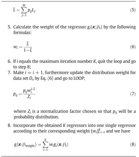
Assume that the process variable and target variable matrices X and Y are stored pair-wise in the history database.As we see in Fig.2,a required number of query points are selected within the latestyfeedback cycle.For simplicity,the number of the query points is usually set to be the same as that of missingyvalues.And for each of those query points,the JIT module estimates the correspondingyvalue.All those estimatedyvalues construct the latest part of the new moving window,i.e.the ‘blk3’.As forhow the JIT-based estimation is performed,it is simple that given a query point xqwe firstcollect from history database certain number of most similar candidate data points by computing the similarity between history data points and the query point.With similar data points collected,the JIT-based estimation is performed by the weighted average of all theyvalues of those collected data points.The whole procedure can be expressed by the formulas listed below.

Fig.2.Illustration of the schematic diagram.

wheredjmeasures the similarity between history data and the query point,σdis the approximated standard deviation of{dj}and λ is a parameter that controls the decay rate of ωjof different distancedj.In Eq.(3)ldenotes the number of the data points selected for a single query point.Eq.(1)computes the similarity to obtain the data points and Eq.(2)assigns for each of the data points a weight according to the distance to the estimated ‘center’of the collected data points.Significantly Eq.(3)performs the estimation of all theyvalues for the query points.

According to the schematic diagram in Fig.2,now that we have obtained the initially estimated values for the ‘blk3’,a new MW of target variableyis constructed by removing the data of the ‘blk1’and adding data of the ‘blk3’to the ‘blk2’as illustrated in Fig.2.The ‘blk1’and‘blk2’are initially constructed by the field feedback values ofy.The‘blk1’is removed because it contains data of the oldesty-feedback cycle and comparatively contributes the least to the currentyvalue.The next step is to transfer the new MW to the AdaBoost module to finally obtain a local estimator within the local region covered by the new MW.Note that this local estimator differs from the soft sensor model.specifically it is notourattemptto obtain an approximated fragment of the softsensor model over this region.Instead,we take the new MW as a normal data set{(X,Y)}MWwhich represents certain potential parameterized modelg(x;β)of input variables x,characterized by parameters β={β1,β2,…}.In another way,the local estimator is exactly the parameterized model.The purpose of this parameterized model is to re-estimate the ‘blk3’,which is discussed in later part.

Let us first give some presentation of the AdaBoost-based regression.AdaBoost-based regression is a kind of boosted regression,which is a powerful machine learning technique for regression and classification problems[16-18].The main idea of boosted regression is to obtain a predictor in the form of an ensemble of multiple weak predictors.It has been demonstrated theoretically that compared with many other machine learning methods the AdaBoost-based method suffers little from the over fitting issue and performs robustly dealing with noisy data as well.Considering that the data source involved in our study is inevitably troubled by uncertainty and noise,we decided to adopt the AdaBoost-based method to process related data set.

The main working mechanism of the AdaBoost module is visualized in Fig.3.As shown in the schematic diagram,the AdaBoost module processes input data set of the new MW.For simplicity,let us denote the data set of the new MW asDx.As shown each data ofDxis assigned an equal weight initially.The weight determines the chance of being sampled.According to the weight we sample fromDxwith replacement to obtain a training setDx1and then use the training set to train a regressor.As shown in the figure,a prediction loss assessment is designed to assess the trained regressor and calculate a weightw1for the regressor.The main function of the assessment is to adjust the weights for data setDx.For a particular member of the data setDx,the larger the prediction error is,the larger the weight of that member is assigned.The interpretation of the way of weight adjustment is that data point with large prediction error represents the weakness of the regressor and more attention shall be paid to fix it in the next round.As the weights of data set change,the chance of being selected in the next round is also changed for each member ofDx.By repeating the above procedure,we are capable to train certain number of regressors{g(x;βi)}.These trained regressors usually have weak performances,but the magic of the AdaBoost regression is reflected by making a weighted combination of these weak regressors so as to obtain a powerful regressorg(x;βweight).Assume that the ultimate powerful regressorg(x;βweight)is obtained.The data set of‘blk3’is reestimated by the ultimate regressor for re fining and next the reestimated ‘blk3’is then used to calibrate the soft sensor model by adjusting the model's parameters.In this way the soft sensor model is calibrated regularly to maintain its performance.For a better understanding,we specifically presented the details of the adjustment of the soft sensor model's parameters.We usef(x,θ)to represent the soft sensor model as shown in Fig.2.In orderto online update the parameters with the continuously obtained data set,we de fine an instantaneous risk function by

wherel(f(x,θ),y)de fines the loss function andacts as the penalty term.Commonly the process of the adjustment of the model's parameters can be conducted by the stochastic gradient descent method,which is given as below.

Adjustment of the model's parameters

To draw a conclusion,when there is no field feedback of the target variabley,we use the proposed calibration method to calibrate the soft sensor model.Otherwise,we directly use the field feedback values ofyto calibrate the soft sensor model.The main procedure of the AdaBoost module is given below.

Procedure of the AdaBoost module

(continued on next page)

(continued)

2.2.The advantage of the calibration method

From the perspective of modeling the proposed calibration method involves the MW-based modeling and the JIT-based modeling.In another way,the calibration method is considered as the cascade of the MW-based model and the JIT-based model.Reasonably the proposed method should have advantages over the MW-based method and the JIT-based method when deployed alone respectively.

The MW-based modeling is commonly applied in scenarios such as online building or maintaining ofsoftsensors,process modeling and online process monitoring[19,20].The idea behind it is to use a moving window consisting of a series of history data to analyze and predict the trend of the target variable.Note that the soft sensor model is basically an approximation of the target process within certain application domain.That means the performance of the soft sensor can be guaranteed within the domain and deteriorates or even malfunctions outside the domain.The generalization ability of the soft sensor is of great significance during its service.Because the soft sensor model is usually built based on finite number of training data,the generalization ability over other new data points other than those training data points is always an important issue.The relationship between the accuracy of prediction of the soft sensor and the application domain is studied by Japanese scholar Hiromasa[3].According to their study,the prediction accuracy is directly affected by the distance between the testdata points and the training data points.The idea behind their study is that the prediction accuracy on the test point is poor if the distance is large andvice versa.As we can see in Fig.4(a),point B is nearer to point A than point C and correspondingly the variation and trend of target variable within the I-zone are milder and smoother than the II-zone,which means that the prediction uncertainty of the I-zone is much smaller than that of the II-zone.Comparatively the situation of the II-zone is‘beyond expectation’,i.e.poorly predictive.Note that they-feedback cycle is much larger than the x-feedback cycle.This consequently leads to a dilemma that the available training data set is highly sparse.Under such a circumstance,for new data points scattering within the large gaps between the training points,the distance between a majority of new data points and the training data points is inevitably large.And we may use the concept of gap andy-feedback cycle interchangeably in the rest part of the paper.The concept of gap is simply interpreted as they-feedback cycle.As a result,there is too much uncertainty for the prediction of the variation of the targetywithin a considerably largey-feedback cycle.Let us discuss the performance of the MW-based method under the above circumstance.As we can see in Fig.4(b)the gap between the two neighbor points consists of many missing target variableyvalues.When we build a MW-based model for estimation,the model reasonably performs well within a neighborhood around those training data points.As shown in Fig.4(b),the neighborhood is represented byd_effect(k).Obviously for those missing points ofy,if the distanced(i,k)to the closest training point is larger than thed_effect(k),the accuracy of estimating that missing data point is not guaranteed.Therefore,when they-feedback cycle is considerably large,the performance of directly using the MW-based method to estimate missingyvalues is commonly poor according to the study of Hiromasa.

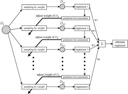
Fig.3.Schematic diagram of AdaBoost regression.

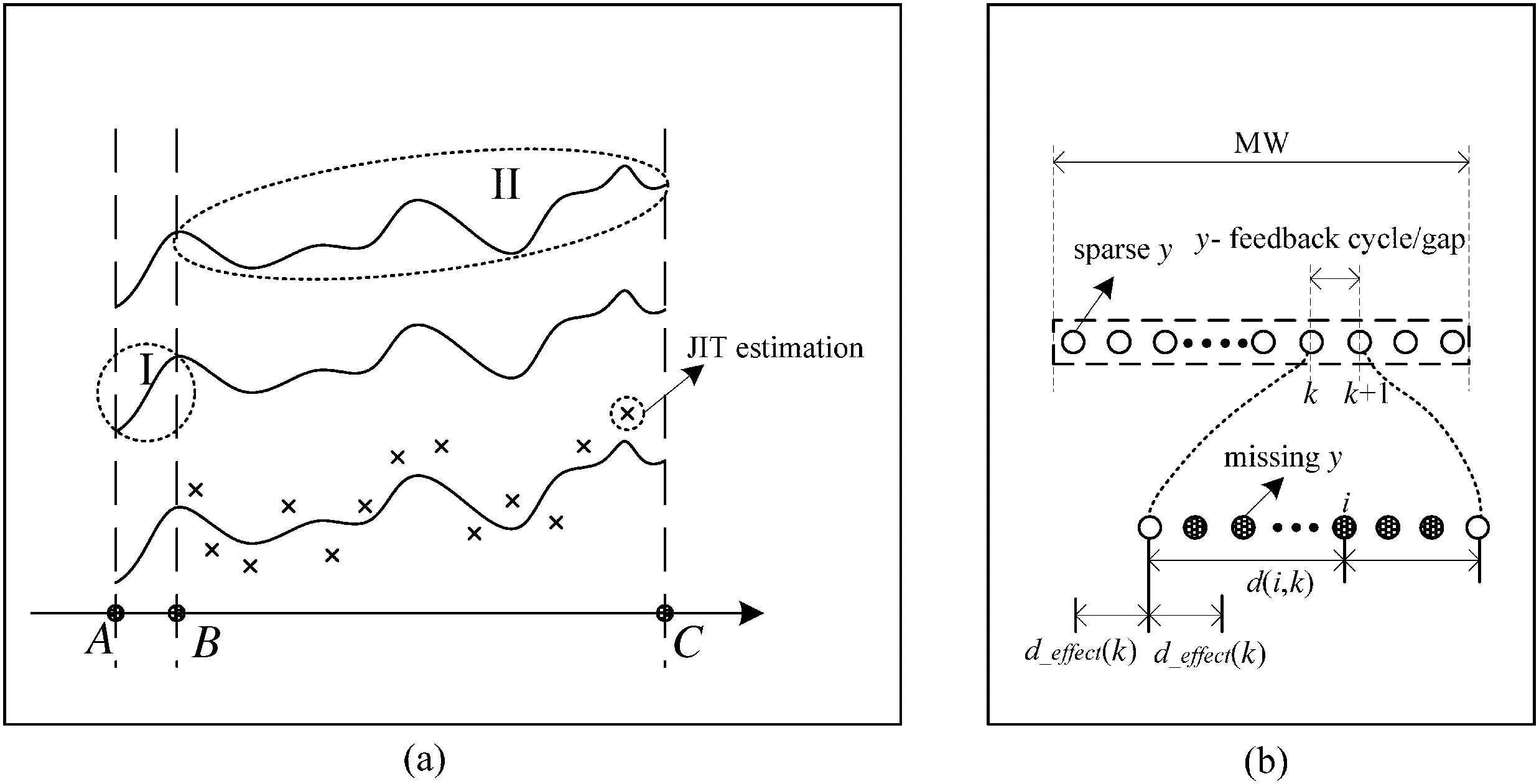
Fig.4.(a)Uncertainty of prediction and drawback of JIT,(b)drawback of MW.

Apparently to solve the problem,a possible and effective solution is to improve the sparsity by interpolation over they-feedback cycle.In such a way,the prediction accuracy of the variation of the target variableycan be increased in some way.Speaking of interpolation over they-feedback cycle,JIT-based modeling can naturally handle the work as we have discussed its mechanism previously.Here is how we perform the interpolation by JIT-based method over ay-feedback cycle:we first pick as many anchor points as the missing data points and use these anchor points as query points for the JIT module.Assume that the missing targetyvalues of those anchor points are estimated.There comes a problem that if we can directly use these estimated values for the calibration of soft sensor model,which,however,is not the strategy of our proposed calibration method.Note that the performance of the JIT-based method is directly affected by the quality of the used history database.As a result,the accuracy of the estimated targetyvalue corresponding to the query point xqcannot be guaranteed.For a better understanding,let us look back into Fig.4(a).The crosses in the figure represent the coarsely estimated missingyvalues by the JIT module.These estimatedyvalues fluctuate around the real values with significant deviations.If we directly use these values to calibrate the soft sensor model,it is likely that the model parameters will change fiercely orthat the calibration will be misguided in some way.Therefore it is not a good choice to directly use the JIT-based method for the soft sensor calibration,especially when we cannot guarantee the quality of the history database.

Although it is not our strategic choice to directly use JIT-based method for the calibration,these estimatedyvalues by JIT module can indicate the variation or the trend of the target variableycoarsely.After all,the philosophy is that it is better than nothing.Our proposed calibration method adopts the JIT's estimation as important prior information on those missingyvalues.Basically we can conclude that the MW-based method has reliable data but suffers from data sparsity while the JIT-based method can obtain sufficient data but has the problem of data reliability and accuracy.The strategy is to mix these coarseyvalues with many history values of realyfeedback to improve the data sparsity of the MW.In such a way we actually take the advantages of both the MW-based method and the JIT-based method.The idea behind it is that the proposed method uses the JIT's estimation to improve the uncertainty of prediction over the gap while uses the MW's field feedback data to balance the unreliability of the JIT-based method.Theoretically the proposed calibration method shall perform better or at least no worse than the two methods.

Fig.5.Illustration of the construction of the MW.

The new MW consists of the ‘blk2’and the ‘blk3’.As the calibration method runs,the ‘blk2’is constructed by the field feedback values ofyand re fined estimation of the missingyvalues,and the ‘blk3’containsy's coarse estimations by the JIT module before reestimated by the AdaBoost module.For a better understanding,a necessary complementary presentation of the MW's construction is visualized in Fig.5.As shown in the figure theyvalues of the ‘blk3’are reestimated for re fining.On the one hand,these reestimatedyvalues are finally used to adjust the parameters of the soft sensor model for calibration.On the other hand,the old ‘blk3’is replaced by the reestimated one.Intuitively we are more con fident of the reestimated ‘blk3’and use it as the latest part of the new MW.In such a way,as the MW slides,the MW can comparatively be ranked as reliable by taking in not only those sparse field feedback values of target variableybut also the many reestimatedyvalues of ‘blk3’.As we can see the ‘blk2’is made up of field feedback values ofyand the re fined estimated values of missingy.This in turn leads to considerably reliable re-estimation of‘blk3’in which we can have a high belief.In another way,there runs a positive circle during the service of the proposed calibration method.

Fig.6.Illustration of(a)pH neutralization facility,(b)schematic diagram of the pH neutralization facility and(c)pH neutralization curve.

3.Case Studies

Because the proposed calibration method can be viewed as the combination of the MW-based method and JIT-based method,the proposed method should possess the advantages.In this section,we conducted some comparative experiments on a real pH neutralization facility to prove the feasibility and superiority of our method.

The pH neutralization reaction is a typical and important process used widely in both industrial scenarios and laboratory.Fig.6(a)shows the main part of the experiment facility in our laboratory.As we can see,the facility has three plastic barrels,four pulse pumps and a reaction tank in the upper right.The three barrels are for acid solution(H2SO4),alkali solution(NaOH)and waste solution,respectively.Only three pulse pumps are used for pumping acid,alkali and waste solution with the fourth pump spared.The reaction tank is where pHneutralization proceeds.As illustrated in Fig.6(b),the acid solution and alkali solution are pumped into the reaction tank where a stirrer keeps stirring to facilitate the neutralization reaction.When the level of the waste solution is high,the waste solution pump starts to work.

Now let us give the characteristics of this process.The characteristic curve of the pH neutralization reaction is given in Fig.6(c).Obviously this process suffers from high nonlinearity,especially when the pH value is around 7.0.We give the mechanism model of pH neutralization reactor as below[21].

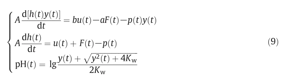
where pH(t)is the pH value;h(t)is the level of the reactor;y(t)is described asy(t)=[OH-]-[H+];u(t),F(t)andp(t)are alkali pump flow,acid pump flow and effluent flow,respectively.A,a,bandKware constants:Ais the base area of the reactor;aandbare the concentrations of acid and alkali solutions,respectively;Kwis the water equilibrium constant andKw=10-14.

Fig.7.Benchmark data of pH value used for the comparative experiments.

Fig.8.Experimental results with cycle ratio set to be 50.

When the pH neutralization reaction runs,the data stream of the process variables and the target variable is stored in the PHD(Honeywell Process History Database)database.They-feedback cycle of the pH value and the x-feedback cycle of the process variables are originally set to be 1 s.However,during the experiments they-feedback cycle can be set larger than 1 s as needed.Let us introduce the concept of cycle ratio.The cycle ratio is de fined as the ratio ofy-feedback and x-feedback.If they-feedback cycle is larger than x-feedback,the cycle ratio is greater than one.Obviously the situation our study encounters is that the cycle ratio is usually much larger than one.Conventionally it is necessary and persuasive to conduct comparative experiments under the same experimental conditions.Therefore,the comparative experiments in this paper were performed by calibrating the same soft sensor model with the same cycle ratio over the same benchmark test data to obtain a comparison of the calibration performances.Note that the nonlinearity of the pH neutralization around 7.0 is highly severe.We decided to collect the benchmark test data around 10.0.As shown in Fig.7,a total of 2000 data over 2000 s were collected as the benchmark data for the experiments.A kind of soft sensor model derived from the Wiener structure is proved effective with cycle ratio set to be one over the pH neutralization test data[22,23].Thereby the soft sensor model used for our comparative experiments was chosen to be the Wiener-based model.For the comparative group,the MW-based method is implemented a MW-based regression model and the JIT-based method is implemented a JIT-based PLS regression model.The number of training data used to train both the MW-based regression model[19]and the JIT-based PLS regression model[9]is set to be 50.The criterion used to assess the calibration performance is the rootmean-square-error(RMSE)calculated with 100 data where each calibration method predicts the correspondingyvalues.

Initially the cycle ratio was set to be 50 for the comparative experiment.The experimental results are illustrated in Fig.8 among which the figure of(I)is an overview of the comparison of calibration performances of the three calibration methods and the figure of(II)is the specific comparison of JIT-based methodversusthe proposed calibration method and MW-based methodversusthe proposed calibration method.The results show that the overall calibration performance of the proposed calibration method is much better than that of both the JIT-based method and the MW-based method.Thereby the results in turn verified the theoretical feasibility and advantages of the proposed calibration method.

As the cycle ratio(still greater than one)changes,the performance of the calibration method will also change.Intuitively it is required and interesting to study how the performance changes as the cycle ratio.We conducted a series of comparative experiments to have a visualized view into the potential relationship.During the experiments,we set the cycle ratio to be from 20 to 200 in steps of 10.For each of the cycle ratios,we calculated the RMSE values over the 2000 data.In such a way,we managed to obtain experimental results presented in Fig.9.By looking into the three figures,we can easily see that the calibration performances of all the three calibration methods deteriorate as cycle ratio rises and that comparatively the proposed calibration method performs the best while the JIT-based method performs better than the MW-based method to some extent especially when cycle ratio is considerably large.The results apparently make sense.As cycle ratio rises,theoretically the variation of the target variableywithin the gap becomes less and less predictive.As discussed previously the serious sparsity will rapidly weaken the prediction performance of the MW-based method though the MW uses more reliable data than the JIT.Although the advantage of JIT-based method is its ability to obtain sufficient estimated data for prediction,the JIT's estimated data over the gap lack sufficient reliability.Hence,when the cycle ratio is relatively small,the MW-based method performs better than the JIT-based method.Contrarily the JIT-based method begins to perform better than the MW-based method as the cycle ratio becomes considerably larger.Comparatively the proposed method takes advantages of the MW-based method and the JIT-based method and achieves a considerably satisfactory calibration performance.Therefore,we can conclude that the proposed calibration method is feasible and effective in cases where they-feedback cycle is much larger than the x-feedback cycle,i.e.the cycle ratio is considerably large.

Finally a summarization of the results of the comparative experiments is given in a table for a clear visualization.For simplicity,we denote the cycle ratio asrand usepprop,pJITandpMWto represent the performance of the proposed calibration method,the JIT-based calibration method and MW-based calibration method,respectively.

Note:↓represents decrement.

4.Conclusio ns

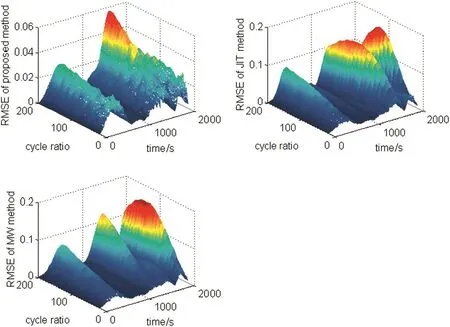
Fig.9.Experimental results under different cycle ratios.

In most industrial processes soft sensor are widely applied.However,soft sensor cannot be calibrated timely and consequently the performance gradually deteriorates due to the lack of sufficient feedback values of the hard-to-measure target variabley.To solve the problem,we proposed a soft sensor calibration method by using JIT modeling and AdaBoost learning method.The proposed calibration method is basically the combination of the MW-based method and the JIT-based method and theoretically should perform better than the two methods.

The feasibility and effectiveness of the proposed calibration method is verified through a series of comparative experiments under different values of cycle ratio on a pHneutralization facility in our laboratory.The experimental results show that the proposed method has a better calibration performance than the MW-based method and the JIT-based method as the cycle ratio rises.But there is a problemthat the field feedback of target variableyis assumed reliable.However,the reliability of the feedback can be weakened by the fault or drift of field sensors or they-analyzer.In addition,if the history database used by the JIT method is badly corrupted,the feasibility of JIT method can be ruined.With the problem taken into account the performance of the proposed calibration method will be greatly challenged.Thereby our future study will include the influence caused to the calibration method by the above problem and the solution to solve the problems.

[1]L.Fortuna,S.Graziani,A.Rizzo,M.G.Xibilia,Soft sensors for monitoring and control of industrial processes,Springer,London,2007.

[2]P.Kadlec,B.Gabrys,S.Strandt,Data-driven soft sensors in the process industry,Comput.Chem.Eng.33(4)(2009)795-814.

[3]K.Hiromasa,A.Masamoto,F.Kimito,Applicability domains and accuracy of prediction of soft sensor models,AIChE J.57(6)(2011)1506-1513.

[4]X.Zuo,F.Tu,H.Y.Qing,X.L.Luo,Advanced control of acetylene hydrogenation reactor(II).Soft sensor and its engineering practice,Control Instrum.Chem.Ind.(China)30(2)(2003)19-21.

[5]R.Feng,Y.J.Zhang,Y.Z.Zhang,H.H.Shao,Drifting modeling method using weighted support vector machines with application to soft sensor,Acta Automat.Sin.30(2004)436-441.

[6]J.J.Macias,P.Angelov,X.W.Zhou,A method for predicting quality of the crude oil distillation,Proceedings of the Int.Symp.Evolving Fuzzy Syst,Lake,United Kingdom 2006,pp.214-220.

[7]X.Wang,U.Kruger,G.W.Irwin,Process monitoring approach using fast moving window PCA,Ind.Eng.Chem.Res.44(2005)5691-5702.

[8]P.Kadlec,B.Gabrys,Adaptive local learning soft sensor for inferential control support,Proceedings of the Int.Confer.Comput.Intel.Modelling Contr.Auto.Vienna,Austria 2008,pp.243-248.

[9]H.P.Jin,X.G.Chen,J.W.Yang,L.Wu,Adaptive soft sensor modeling framework based on just-in-time learning and kernel partial least squares regression for nonlinear multiphase batch processes,Comput.Chem.Eng.71(2014)77-93.

[10]S.Khatibisepehr,H.Biao,F.W.Xu,A.Espejo,A Bayesian approach to design of adaptive multi-model inferential sensors with application in oil sand industry,J.Process Control22(2012)1913-1929.

[11]G.Cybenko,Just-in-time learning and estimation,in:S.Bittanti,G.Picci(Eds.),identification,adaptation,learning:The science of learning models from data,Springer,Berlin 1996,pp.423-434.

[12]C.Cheng,M.S.Chiu,A new data-based methodology for nonlinear process modeling,Chem.Eng.Sci.59(13)(2004)2801-2810.

[13]K.Fujiwara,M.Kano,S.Hasebe,A.Takinami,Soft-sensor development using correlation-based just-in-time modeling,AIChE J.55(7)(2009)1754-1765.

[14]S.Kim,M.Kano,S.Hasebe,A.Takinami,T.Seki,Long-term industrial applications of inferential control based on just-in-time soft-sensors:Economical impact and challenges,Ind.Eng.Chem.Res.52(35)(2013)12346-12356.

[15]Z.Ge,Z.Song,A comparative study of just-in-time-learning based methods for online soft sensor modeling,Chemom.Intell.Lab.104(2010)306-317.

[16]R.E.Schapire,Explaining adaboost,Empirical inference,Springer,Berlin Heidelberg 2013,pp.37-52.

[17]R.Rojas,AdaBoost and the super bowl of classifiers a tutorial introduction to adaptive boosting,Freie University,Berlin,Tech.Rep,2009.

[18]Y.Freund,R.Schapire,N.Abe,A short introduction to boosting,J.Jpn.Soc.Artif.Intell.14(1999)771-780.

[19]Y.Liu,N.Hu,H.Wang,et al.,Soft chemical analyzer development using adaptive least-squares support vector regression with selective pruning and variable moving window size,Ind.Eng.Chem.Res.48(12)(2009)5731-5741.

[20]S.J.Qin,Recursive PLS algorithms for adaptive data modeling,Comput.Chem.Eng.22(4)(1998)503-514.

[21]X.L.Luo,Process of fluid flow,Chemical process dynamics,Chemical Industry Press,Beijing 2005,pp.25-27.

[22]P.Cao,X.Luo,Modeling for soft sensor systems and parameters updating online,J.Process Control24(6)(2014)975-990.

[23]P.F.Cao,X.L.Luo,Softsensor model derived from Wiener modelstructure:Modeling and identification,Chin.J.Chem.Eng.22(5)(2014)538-548.