A continuous-time formulation for re finery production scheduling problems involving operational transitions in mode switching☆

Lei Shi,Yongheng Jiang ,*,Ling Wang ,2,Dexian Huang ,2

1 Institute of Process Control Engineering,Department of Automation,Tsinghua University,Beijing 100084,China

2 Tsinghua National Laboratory for Information Science and Technology,Tsinghua University,Beijing 100084,China

1.Introduction

Production scheduling is essential to improve the operation and management and achieve better economic performance for re fineries.Short-term scheduling of re finery operations is one of the most challenging problems due to the complexity of production process.The research area has received considerable attention and various publications in scheduling models and approaches based on continuoustime formulations have appeared in the past two decades.Ierapetritou and Floudas[1,2]presented a continuous-time formulation for the short-term scheduling of multipurpose batch processes,continuous and semicontinuous processes,giving simpler models with plant characteristics accommodated easily.Pintoet al.[3]presented a nonlinear planning model for re finery production,with the scheduling problems formulated as mixed-integer optimization models.Based on the resource-task networks(RTNs),Castroet al.[4]presented a general mathematical formulation for scheduling multipurpose plants involving batch and/or continuous processes.Jia and Ierapetritou[5]developed a comprehensive mathematical programming model for oilre finery operation scheduling based on a continuous-time formulation.Castro and Grossmann[6]proposed a multiple-time-grid continuous-time MILP model for short-term scheduling of multistage,multiproduct plants and provided a critical review of other approaches for this type of scheduling problem.It is pointed out that there is not an ideal approach for all types of problems and objective functions.Mouretet al.[7]proposed a new continuous-time formulation to address crude-oil scheduling problems and used a simple two-step procedure for an MILP and an NLP to solve the MINLP model.Shah and Ierapetritou[8]presented a comprehensive integrated optimization model based on a continuous-time formulation for scheduling production units and endproduct blending.Besides these specific examples,some excellent reviews were published.Floudas and Lin[9]presented an overview on discrete-time and continuous-time approaches for scheduling of chemical processes,with computational studies and applications.Panet al.[10]reviewed continuous-time approaches for short-term scheduling of network batch processes and solved several benchmark examples with different models to evaluate their performance.Harjunkoskiet al.[11]presented a review on the existing scheduling methodologies developed for process industries and discussed modeling of time in detail.all these researches are valuable and meaning ful For the development of re finery scheduling.Nonetheless,the realization of operation modes and the transient behavior between different operation modes have not been discussed.

Different operation modes result in diversities of yields and properties of products and operational costs of processing units.For production units with more than one operation mode,mode switching in the scheduling horizon is inevitable.In many papers,penalties are adopted to calculate the cost of mode switching in the objective function.However,because of the large inertia characteristic of continuous process industry,the switching cannot be accomplished instantly.To reflect the time factor in these scheduling problems,operational transitions have to be considered.Dimitriadiset al.[12]provided necessary theoretical basis for exploitation of partial resource equivalence,which allows large RTNs to be reduced to smaller but completely equivalent ones.Such reductions are particularly significant in problems involving many sequence-dependent changeovers.Limaet al.[13]addressed the long-term scheduling of multi-product single stage continuous process for manufacturing glass and proposed several new features,including minimum run lengths and changeovers across due dates.Mitraet al.[14]presented an optimal production planning for continuous powerintensive processes under time-sensitive electricity prices,described a discrete-time deterministic MILP model,and emphasized the systematic modeling of operational transitions,which result from switching the operating modes of plant equipment.The transitional modes help capture ramping behavior and obtain practicalschedules.The transition cost is involved in the objective function.

It is a big challenge to set up realizable and industrially meaningful operation modes for re finery scheduling problems.In ourgroup's previous research,Lvet al.[15]have proposed a new strategy for integrated control and on-line optimization on high-purity distillation process.The split ratio of distillate flow rate to that of bottoms is used in a new predictive control scheme as an essential controlled variable.With the strategy,the process achieves its steady state quickly.Based on the unit-wide MPC, finite optimal operating modes for units are realized.Shiet al.[16]have proposed a re finery scheduling model,which involves operational transitions in mode switching based on the discrete-time representation.The operation modes in the model are de fined based on special unitwide predictive control,so they are realizable and applicable.The scheduling model can formulate the dynamic behavior of production more accurately by involving transitions of mode switching.The advantage of discrete-time approach is that it is convenient to describe the constraints of mode switching.Shiet al.[17]have reformulated the discrete-time model in[16]by rede fining the binary variables describing operation modes and transitions.Bilinear and trilinear terms in the objective function and constraints are no longer needed and the size of the primal model can be reduced.The reformulation can improve the solving efficiency significantly.However,as the scheduling time intervals increase,it leads to very large scale combinatorial problems,which are difficult to solve.And the definition of timeline in the discrete-time formulation is an approximation of the actual problem.Compared with the discrete-time representation,the continuous-time representation needs relatively less variables and constraints in some cases and the processes can run for a time period of any duration.

In this paper,we propose a novel model for the whole re finery operations based on the continuous-time representation.The control system is the basis of re finery scheduling.A well-organized scheduling scheme can help the implementation of the control system.Compared with the models in previous work,the transitions of mode switching are involved in this model for a more detailed description of dynamic behavior in the process.Then the implementation of the scheduling schemes obtained by the proposed model can be guaranteed.To describe the scheduling model efficiently,the global event-based formulation is used.Both transition constraints and production transitions are introduced and a MILP model is presented.The numbers of key variables and constraints in both the discrete-time and continuous-time models are discussed.

2.Problem Statement

An industrialre finery is studied in this paper.The structure of the refinery is the same as that in the discrete-time scheduling model[16].The overall system is depicted in Fig.1.It can be decomposed into three stages:crude oil feeding,product processing,and blending and delivery.The crude oil is fed from crude oil tanks.The amount of crude oil is sufficient.There are eight production units in the product processing,including atmospheric distillation unit(ATM),vacuum distillation unit(VDU), fluid catalytic cracking unit(FCCU),hydrogen desulfurization unit(HDS),etherification unit(ETH),catalytic reformer unit(RF),methyl tert-butyl ether unit(MTBE unit),and hydro-re fining units(HTU1 and HTU2).The operation modes for production units are shown in Table 1.The yields and operation costs of processing units are shown in Tables A1-A5 in Appendix A.

Because of the large inertia characteristic of the process,the mode switching of units cannot be achieved instantly.If a processing unit changes its operation mode,it will lead to an operational transition between two operation modes.During transitions,the key properties of products will fluctuate,and accumulated indicators will lie between those in the preceding operation mode and the succeeding one.The operation costs in transitions are higher compared with those in the operation modes.For transitions with the same preceding and succeeding operation modes,the transition time is the same,but for transitions with different preceding and succeeding operation modes,the transition time may be different.In this paper,each transition is viewed as a whole.A new transition cannot be started before the previous one ends.To simplify the scheduling model,the operational cost and the yield are calculated averagely in the transitions.

The third part involves the blending and delivery of product oil.There are one kind of crude oil and eight kinds of product oil,including five kinds of gasoline and three kinds of diesel.The key properties of component oils are related with the operation modes of corresponding production units.When the operation mode of a production unit is switched,the key properties of component oil will change accordingly.The product oil is stored in the oil tanks.The objective function is to minimize the total cost of production and penalties.

3.Time Representation

In the discrete-time formulation[16],the scheduling time horizon is divided into a number of time intervals of a given duration.The exact time points are known as prior knowledge.At each time interval,the variables to be determined are operation modes and processing amounts of each unit,amounts and types of component oil consumed in blending,and amounts and types of production oil stored or delivered.The scheduling time horizon in the continuous-time formulation is partitioned into a fixed number of periods,and lengths are to be determined.

Continuous-time representations have been developed significantly in the last two decades.In the review presented by Harjunkoskiet al.[11],the modeling approaches can be divided into two types:precedence-based models and time-grid-based models.The term time-grid-based is to describe all modeling approaches that employ time slot/periods/points/events.The time-grid-based models can be classified to discrete or continuous ones.Continuous time-grid-based models can be subdivided into approaches employing a single common grid across all units and those employing multiple unit-specific grids.

Re fining is a complex continuous production process.There is material mixing or splitting in the production process.In this study,the key factor for re finery scheduling is how to represent the transitions of mode switching.Different modes and transitions have different yields and operation costs,which make the calculations of mass balance and operation costs significantly important.

In this paper,we employ event points in the continuous-time formulation.The beginnings and endings of transitions are considered as events.The global event points are used corresponding to a single common grid across all units.The calculations of mass balance contain two parts:(1)the output amount of each unit at each time point is equal to the input amount at each time point multiplied by the yield;(2)the input of each unit at each time point is equal to the output from its upstream unit at each time point.

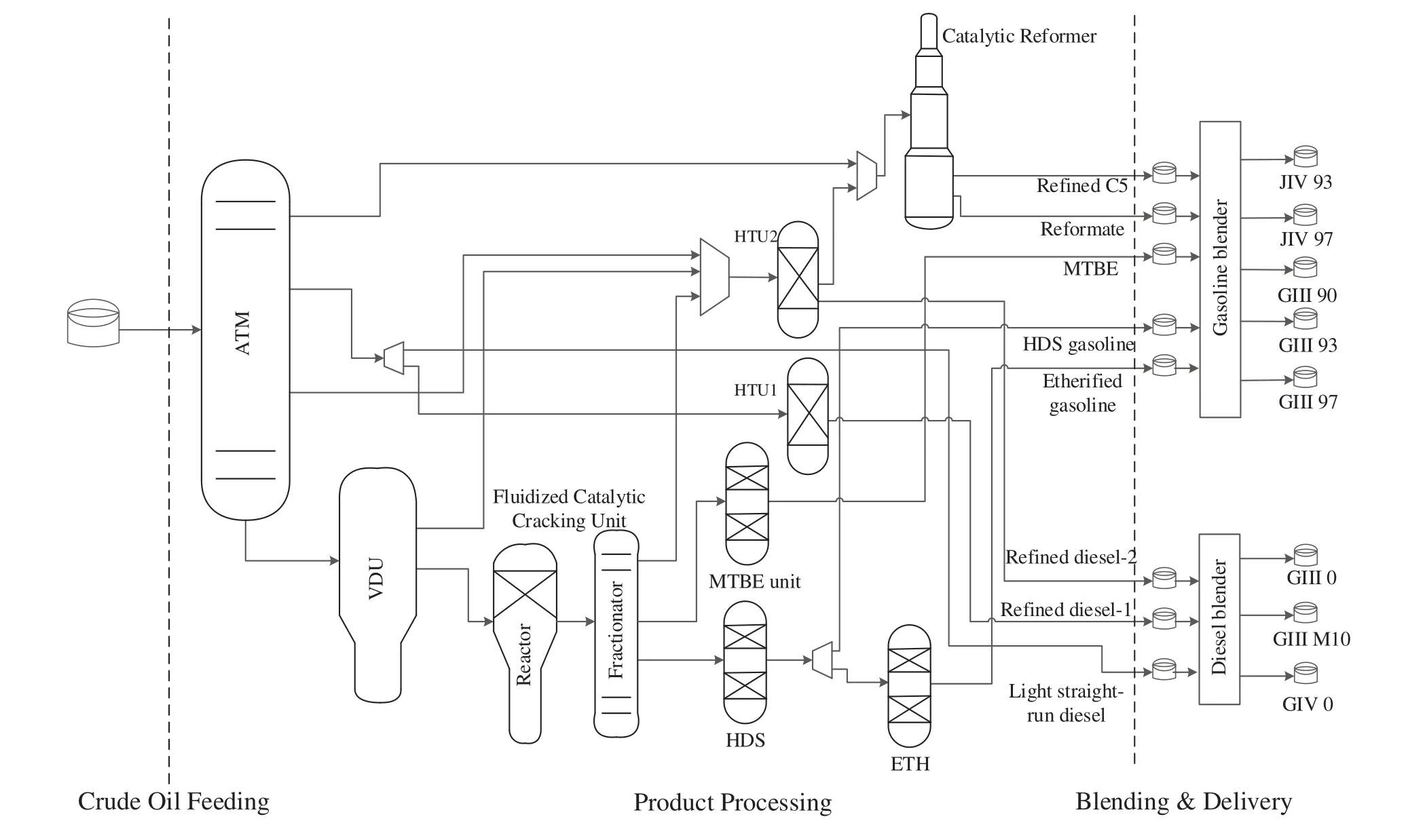
Fig.1.simplified flow sheet of re finery system.

For the scheduling problem in this paper,different binary variables are required to indicate the unit work in an operation mode or in a transition.Some particular constraints such as duration constraints for transitions are also needed.It is convenientto describe these constraints by de fining the beginning and ending of each transition.Three sets of binary variables are introduced.Binary variableswu,m,nrepresent whether unituis in operation modemfrom event pointn-1 ton.Binary variablesdenote whether the transition from operation modemtom′of unitubegins at event pointn.And binary variablesdenote whether the transition from operation modemtom′of unituends at event pointn.According to the definitions of binary variables,if unituworks in the transition from modemtom′at event pointn,the termis equal to one.And if unituworks in the operation modem,binary variablewu,m,nis equal to one.

4.Formulation

In this section,two sets of constraints are included in the continuous-time model.The first set is operation mode constraints for time sequencing,transition variables and operation mode variables.The second set is production constraints for mass balance,capacity,blending and delivery.

4.1.Operation mode constraints

The transitions of mode switching are considered in the scheduling model.To describe mode switching and operation modes in scheduling,the globalevent-based formulation and binary variables are introduced.Some corresponding constraints are required.

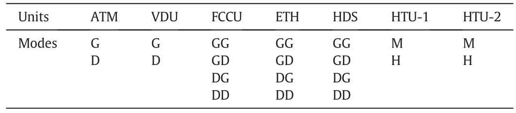
Table 1Operation modes for production units

4.1.1.Time sequencing constraints

Time points keep increasing order.For re fineries,two sequential actions on one unit cannot occur in a certain interval.Tminrepresents the minimum time interval between two neighboring time points.It is a constant from production experience.

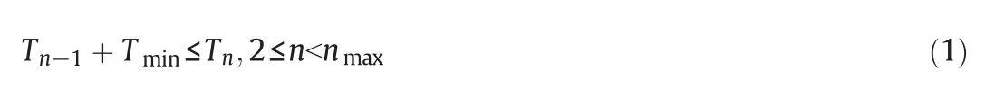
wherenmaxindicates the largest number ofn.

From constraint(1),there is a constraint for the first event point.

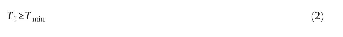
The last event point is designated to the ending of time horizon.The time of the last event point is fixed as the time horizonTH.

4.1.2.Transition variable constraints

The definitions of binary variablesandare the foundations of transition expressions in the scheduling model.=1 means that at event pointn,the operation mode of unitubegins to switch frommtom′.And=1 means that at event pointn,the transition from operation modemtom′of unituends.If=1 and=1,the duration of transition is fromTntoTn′.

For the transitions,we have the following constraints.

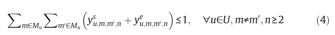
At most one beginning or ending of a transition of each unit can be assigned to the same event point.Muis the set of operation modes for unitu.

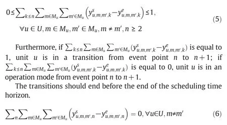
The beginnings and endings of transitions should be alternate for each unit.

4.1.3.Operation mode variable constraints

Besides binary variablesand,binary variableswu,m,nare also needed,which denote the operation modes of each unit at each event point.The constraints forwu,m,nare as follows.

Each unit cannot be in two different operation modes at two neighboring time points.There must be a transition between two different operation modes of a unit.

4.1.4.Transition duration constraints

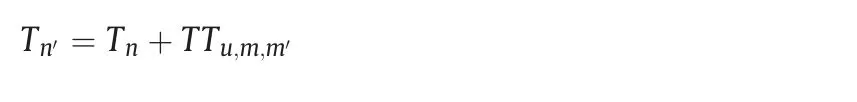
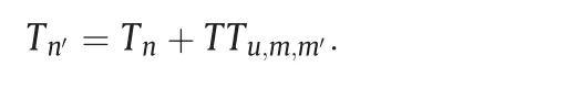
The transition process of unitufrom operation modemtom′involves a fixed duration.TTu,m,m′is used in this model to represent the duration.There cannot be a new mode switching before a transition ends.If the operation mode of unitubegins to switch from operation modemtom′at event pointnand the same transition ends at event pointn′,there is a constraint betweenTnandTn′.

Here we use generalized disjunctive programming[18]to present the transition duration constraints.

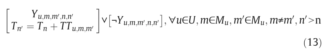
whereTTu,m,m′indicates the length of the transition from operation modemtom′of unitu.Operator“∨”means logical disjunction and operator“¬”means logical negation.

Binary variableYu,m,m′,n,n′indicates if the operation mode of unitubegins to switch from operation modemtom′at event pointnand the same transition ends at event pointn′.We have the following constraints to express the condition thatYu,m,m′,n,n′is equal to one.

Constraint(14)means that the operation mode of unitubegins to switch from operation modemtom′at event pointnand ends at eventpointn′.And constraint(15)indicates that there are notany transitions begin or end at event pointsn+1 ton′-1.Thus the transition from operation modemtom′of unitubegins at event pointnand ends at event pointn′.If constraints(14)and(15)are satis fied,we have the relationship betweenTnandTn′:

Otherwise,ifYu,m,m′,n,n′is equal to zero,there is no certain relationship betweenTnandTn′.

Constraint(13)can be reformulated into the following bigMinequalities.

4.2.Production constraints

We use continuous variablessQIu,m,nandtQIu,m,m′,nto representthe input amountof unitufrom eventpointn-1 tonin operation modemand the transition from operation modemtom′,respectively.

4.2.1.Mass balance constraints

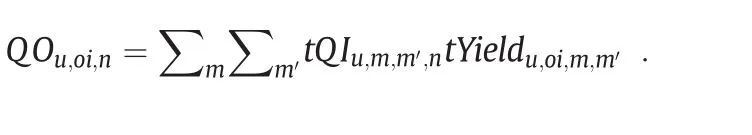
4.2.1.1.Mass balance constraints for outflow ports of units.If a unit involves more than one operation mode,the yield is determined by the current operation mode or transition.The mass balance constraints for output materials are as follows.

whereYieldu,oi,mindicates the yield of component oiloiof unituin the operation modemandtYieldu,oi,m,m′indicates that in the transition from operation modemtom′.

If unituis in an operation mode,tQIu,m,m',nis zero for allmandm′,then the term ∑m∑m′tQIu,m,m′,ntYieldu,oi,m,m′is equal to zero.We have

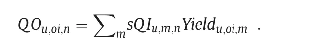
If unituis in a transition,sQIu,m,nfor allmand∑msQIu,m,nYieldu,oi,mis equal to zero.We have

4.2.1.2.Mass balance constraints for intermediate oil.The intermediate oils contain material oils for processing units and component oils for blending.

The mass balance constraints for material oils are written as follows.The constraint represents that the sumof output flow of material oilomfrom upstream units must be equal to the sum of its input flow to downstream units at event pointn.

whereOMindicates sets of material oils.

The mass balance constraints for component oils are as follows.

whereOCindicates sets of component oils.

4.2.1.3.Mass balance constraints for tanks.The inventory of each storage tank at event pointnis equal to that at event pointn-1 plus the amount of flows entering the tank at event pointnand minus the amount of flows leaving at event pointn.

whereINVoc,iniindicates the initial storage of component oiloc,andINVo,iniindicates the initial storage of product oilo.

The relationship betweenQOoc,nandQIo,nis

4.2.2.Capacity constraints

4.2.2.1.Capacity constraints for units.The capacity constraints specify that the average input flow of unituper hour cannot be beyond its lower and upper limits.Since each unit is in a steady state of processing at the beginning of the scheduling time horizon,tQIu,m,m′,1is equal to 0.

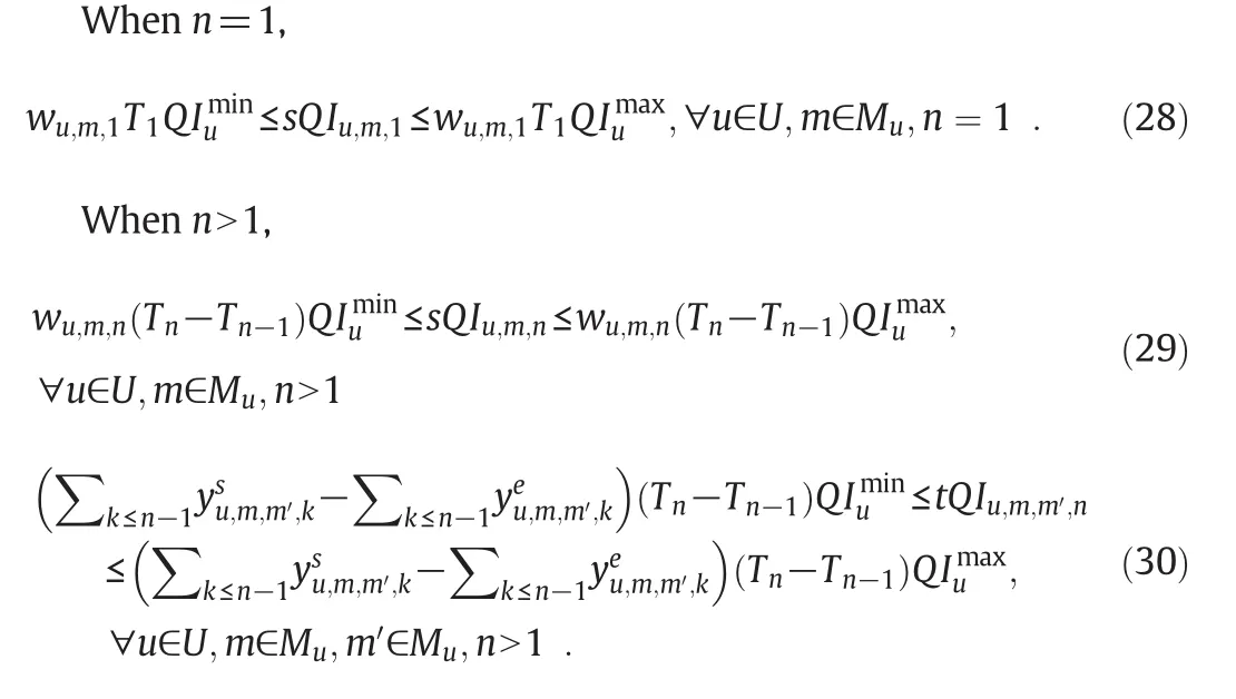
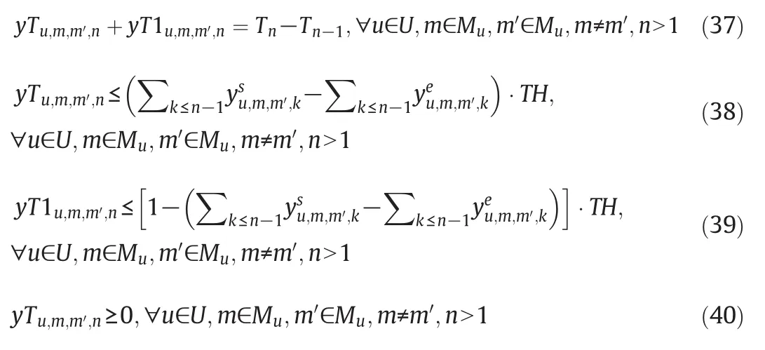
In constraints(28)-(30),bilinear termswu,m,1T1,wu,m,n(Tn-Tn-1),binary term and a continuous term.You and Grossmann[19]have presented a reformulation method for these bilinear terms by introducing auxiliary variables.To linearize these terms,auxiliary constraints are introduced as follows.wTu,m,n,wT1u,m,n,yTu,m,m′,nandyT1u,m,m′,nare auxiliary continuous variables.

Constraints(33)-(36)ensure that ifwu,m,nis equal to zero,wTu,m,nshould be equal to zero;ifwu,m,nis equal to one,wT1u,m,nshould be equal to zero.Combining with constraints(31)and(32),we havewTu,m,1andwTu,m,nequivalent to the product ofwu,m,nandT1orTn-Tn-1whenn=1 orn＞1,respectively.

4.2.2.2.Capacity constraints for tanks.The inventory must lie between its lower and upper bounds.

4.2.3.Blending constraints

4.2.3.1.Product property constraints.The properties of product oil must lie between its lower and upper bounds.Linear rules are adopted to calculate the research octane number(RON)and sulfur content of gasoline,and cetane number(CN)and sulfur content of diesel.The condensation point of blending diesel can also be calculated linearly by introducing the condensation point factor[20].The properties of the flows entering the blenders are connected with the preceding production units.

The constraint can be expressed linearly in an alternative way by multiplying it by∑ocQoc,o,n:

4.2.3.2.Component oil ratio constraints in blending.The component oil consumed in blending has its lower and upper ratios

4.2.4.Delivery constraints

Each order has beginning time and due time For the delivery.Product oil cannot be delivered before the start time or after the due time.The stockout will be penalized.

Dl,o,nis the supply amount of product oilofor orderlat event pointn.Rl,ois the required amount of product oilofor orderl.Tl1is the beginning time of the delivery for orderl.AndTl2is the due time of the delivery for orderl.

Decision variablesydl,o,ndenote whether productoilofororderlcan be delivered at event pointn.Constraints(46)-(48)express that ifTl1≤Tn-1≤Tn≤Tl2,it means that the production fromTn-1toTncan be delivered andydl,o,nis equal to one.

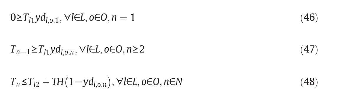
Fig.2 is an example to illustrate the delivery constraints(46)-(48).The delivery for order 1 is from 0 h to 42 h and the delivery for order 2 is from 25 h to 72 h.Based on constraints(46)-(48),the values ofydl,o,nare as follows.

Constraint(49)states that the delivery amountmustlie between the lower and upper amounts of delivery per hour for each product oil.By the definition,ifydl,o,n=0 is equal to zero,Dl,o,nis also equal to zero.

The total delivery amount must be no more than the required amount.

4.3.Objective function

The objective of the scheduling problem is to minimize the totalcost and penalty.Itincludes fourparts:costs ofcrude oil,operationalcosts of units in transitions and operation modes,costs of materialstorages,and penalties of order stockout.All the four parts are described as follows.

4.3.1.Costs of crude oil

According to the simplified flow sheet of re finery system in Fig.1,crude oil feeds ATM.The costs of crude oil are the sum of input flow of ATM multiply by the unit price of crude oil.

4.3.2.Operational costs of processing units

Similarly with constraint(18),operational costs of units consist of those in the operation modes and in the transition processes.

whereOpCostu,mindicates the operation cost of unituin the operation modemandtOpCostu,m,m′indicates that in the transition from operation modemtom′.

Fig.2.Illustration of delivery constraints.

4.3.3.Costs of material storages

Accurate costs of material storages are the integral of the cost that is the storage of each time point multiply by the time duration.

whereαis the inventory costofcomponentoiland productoilper hour.

The term on the right-hand side of Eq.(53)is nonlinear and nonconvex.Jia and Ierapetritou[5]presented an approximate method to calculate the inventory cost linearly.The total inventory levels of storage tanks are approximated by the average value of the inventory level of the tanks in the scheduling time horizon.The approximation is as follows.

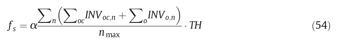
Castro and Grossmann[21]discussed the approximated tank inventory costs in the scheduling ofcrude oilblending operations.They pointed out that the approximate inventory cost is not a good option considering that the optimal number of events is changed for searching the global optimal solution.More specifically,it was observed experimentally that after a certain number of slots,the optimization will“cheat”by duplicating event points corresponding to the points of minimum inventory so that they contribute more to the objective function and the total cost is reduced.To avoid this drawback,in the case study section exact inventory cost is calculated by constraint(53)from the scheduling results to find the best solution.

4.3.4.Penalties of order stockout

The penalties of order stockout are the sum of the stockout of each order multiplied by the penalty factor.The stockout of each order is）Rl,o-∑nDl,o,n）.Constraint(50)makes sure the stockout is non-negative.

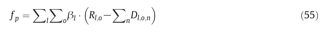
where βlis the penalty for delivery delay of orderlper ton.In summary,the objective function is as follows.

The mixed-integer linear programming model is as follows.

4.4.Comparison of continuous-time and discrete-time scheduling models

4.4.1.Numbers of binary variables

Symbol|s|is used to represent the number of elements in the sets.The binary variables to describe mode switching and transitions in the continuous-time scheduling model areandwu,m,n.The numbers of these variables depend on the values of|Mu|and|N|.

In the discrete-time scheduling model[17],related binary variables arexu,m,m′,tandzu,m,t.Their numbers depend on the values of|Mu|and|T|,which are shown in Table 2.The numbers of binary variables in the continuous-time and discrete-time models are linear functions of|N|and|T|,respectively.

4.4.2.Numbers of constraints

The constraints in the two models can be divided into two parts:transition constraints and production constraints.The transition constraints can be subdivided into transition variable constraints,operation mode variable constraints,and transition duration constraints.The production constraints can be subdivided into mass balance constraints,capacity constraints,blending constraints,delivery constraints,and linearization constraints.The continuous-time modelhas time sequencing constraints in addition.

The numbers of constraints are shown in Table 3.The number of constraints in the discrete-time model is a linear function of|T|and that in the continuous-time model is a quadratic function of|N|.The quadratic term comes from the transition duration constraints.

The continuous-time scheduling model is more complicated than the discrete-time scheduling model.The number of transition constraints in the continuous-time scheduling model has a quadratic term of|N|.However,compared with the discrete-time formulation,the continuous-time representation needs relatively less points to represent the schedule,especially in the cases with large time horizons.Besides,the time period in the continuous-time model can be in any duration.These features may have advantage in the computation.The detailed study is in Section 5.

5.Case Study

In this section,three cases are used to test the proposed continuoustime re finery scheduling model(denoted by “CMT”).The cases are based on a typical re finery in China and the flow sheet is shown in Fig.1.For all the three cases,both the continuous-time model proposed in this paper and the discrete-time model proposed in[17]are solved.For case 1,a continuous-time model involving instant changeovers of operation modes(denoted by “CMnT”)is solved to compare with the proposed continuous-time model.The variations of processing yields and costs in switching are not considered in CMnT.

The cases are solved by CPLEXin GAMS 24.2.2 using a CPUIntelXeon E5-2609 v2@2.5 GHz with RAM 32.0 GB.Sizes of the three cases are shown in Table 4.The key component concentration ranges of productoils are shown in Tables B1 and B2 of Appendix B.The parameters of the scheduling model are shown in Appendix C.

Table 2The numbers of binary variables in the continuous-time and discrete-time models

Table 3The numbers of constraints in the continuous-time and discrete-time models

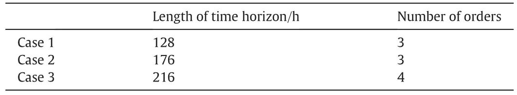
Table 4Sizes of cases

As mentioned in Section 4,the calculation of inventory cost is approximate in the scheduling model by constraint(54).After solving the scheduling model,exact inventory cost is calculated by constraint(53)from the scheduling result.

5.1.Case 1

The orders of product oil for case 1 are in Table 5.The statistics of both continuous-time and discrete-time models are shown in Table 6.The solutions of the two models are shown in Table 7.

In case 1,the length of time horizon is 128 h and the number of orders is 3.The number of eventpoints in the continuous-time model is 7.In the discrete-time model,the time length is 8 h,so the number oftime intervals is 16.The number of variables in the continuous-time modelis about60%of that in the discrete-time model.The number of constraintsin the continuous-time model is about 80%of that in the discrete-time model.The CPU time consumed by solving the continuous-time model is about 1/5 of that for the discrete-time model.From Table 7,we can see that the solution obtained by the continuous-time model is better and the crude oil consumed is less,because the time points in the continuous-time model are flexible,while the events in the discretetime model only occur at fixed time points.

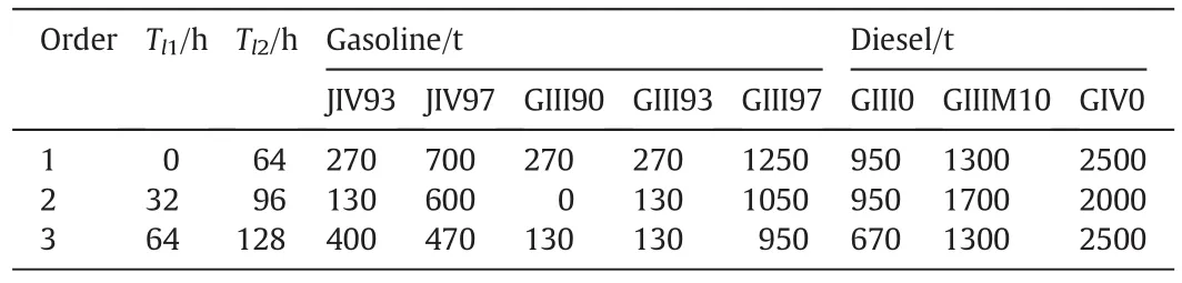
Table 5Orders of product oil(time and quantities)for case 1

The solutions of the proposed continuous-time model and the continuous-time model without considering transitions in mode switching are listed in Table 8.The production schedules ofunits obtained by models CMT and CMnT are shown in Figs.3 and 4.The duration of processing is represented as a rectangle.The transitions are denoted as gray rectangles.The rates of input flow and the operation mode are denoted above and below the rectangles,respectively.In Table 8,the objective value computed by model CMnT is less than that by model CMT,while the objective value of model CMnT in operation is much larger.In Fig.3,the operation modes of ATM are changed four times.That is quite frequent.The mode switching of ATM at time 96 h cannot be realized in actual operation because the operation mode is just switched at time 90.4 h.The ATM needs a duration of 24 h in mode switching(see Appendix C).Also,even if the mode switching can be realized,the processing yields in transitions are lower than those in operation modes.Consequently,the product amounts of intermediate oil will be less than those in the schedule and may cause the order stockout.From Table 8,the objective value of model CMnT in operation is much larger than the computed objective value.In a word,the schedule without considering the transitions will depart from the optimal,even a feasible one.

5.2.Case 2

The orders of product oil for case 2 are in Table 9.The statistics of both continuous-time and discrete-time models are shown in Table 10.The solutions of the two models are shown in Table 11.

Table 6Statistics of continuous-time and discrete-time models for case 1

Table 7Solutions of continuous-time and discrete-time models for case 1

Table 8Solutions of CMT and CMnT for case 1

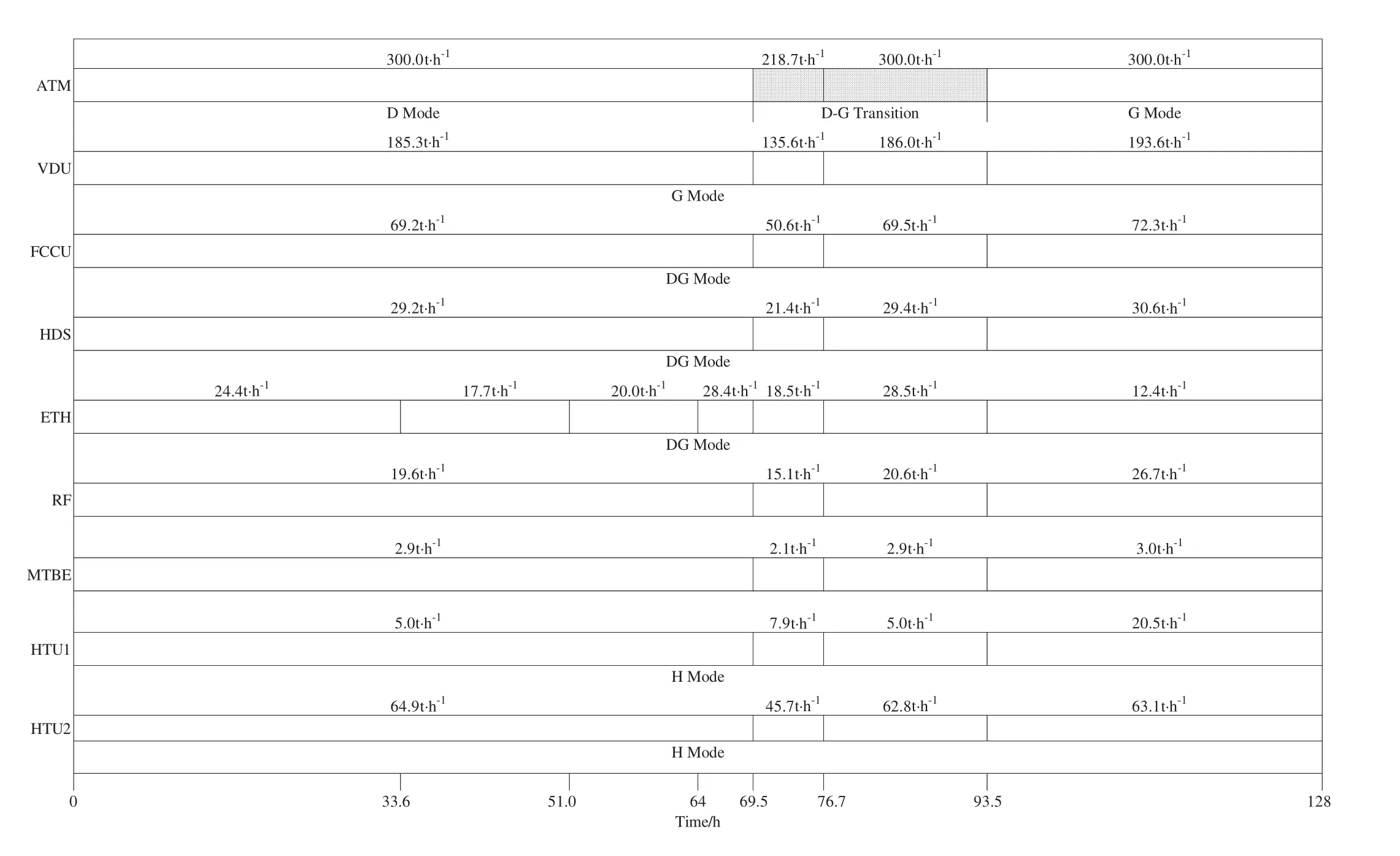
Fig.3.Production schedule of units obtained by model CMT for case 1.

In case 2,the length of time horizon is 176 h and the number of orders is 3.The number of event points involved in the continuous time model is 7,the same as case 1.The length of a time interval in the discrete-time model is fixed,so the number of time intervals increases to 22.The variables and constraints in the continuous-time model are much less.The number of variables in the continuous-time model is about 45%of that in the discrete-time model.And the number of constraints in the continuous-time model is about 60%of that in the discrete-time model.Compared with the scheduling result from the discrete-time model,we can see that the cost of crude oil,the operational cost and the inventory cost of the continuous-time model are all less.This leads to a better objective value.The CPU time consumed by solving the continuous-time modelis about 1/11 of that by solving the discretetime model.

5.3.Case 3

The orders of product oil for case 3 are in Table 12.The statistics of both continuous-time and discrete-time models are shown in Table 13.The solutions of the two models are shown in Table 14.

In case 3,the length of time horizon is 216 h and the number of orders is 4.The number of event points in the continuous-time model is 8.The number of time intervals in the discrete-time model increases to 27.The number of variables in the continuous-time model is about 40%of that in the discrete-time model.And the number of constraints in the continuous-time model is about 60%of that in the discrete-time model.From Tables 13 and 14,we can see that the objective value of the continuous-time model is less and the CPU time is about 1/9 of that for the discrete-time model.Since the time points in the continuous-time model are more flexible,the crude oil consumed in the continuous-time model is less.This makes the objective value of the discrete-time model larger.

5.4.Summary

In this section,we studied three cases with different lengths of time horizons and different numbers of orders to test the performance of the continuous-time and discrete-time models.In case 1,the numbers of variables and constraints in the discrete-time model are larger,which leads to longer CPU time.When the length of time horizon increases as in cases 2 and 3,the scheduling time intervals increase by 1.37 and 1.69 times,respectively,and the CPU time increases by 1.85 and 7.91 times,respectively,with the discrete-time model.Compared with the discrete-time formulation,the continuous-time model involves less variables and constraints for large-scale problems,consumes shorter time to solve the model,and gives better schedules.

Fig.4.Production schedule of units obtained by model CMnT for case 1.

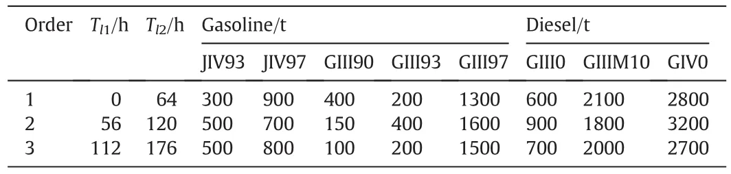
Table 9Orders of product oil(time and quantities)for case 2

6.Conclusion

In this paper,an alternative continuous-time scheduling model for re fineries involving transitions of mode switching is proposed to effectively handle the solving challenge in the present discrete-time refinery scheduling models and obtain better production schedules.The transitions of mode switching are involved in the scheduling model to formulate the dynamic nature of production more accurately.To reduce the difficulty in solving large scale MILP problems resulting from the sequencing constraints,the global event-based formulation is adopted to describe the scheduling model.Both transition constraints and production transitions are introduced and the numbers of key variables and constraints in both the discrete-time and continuous-time formulations are discussed.The effectiveness of the proposed scheduling model is validated by three cases from a typical re finery.The effectiveness of considering transitions is proved by comparison of schedules.Compared with the discrete-time formulation,the continuous-time model usually has less event points and better solving efficiency for large-scale problems,and gives better production schedules.

To solve re finery scheduling problems with longer time horizons and more orders,more event points are needed and the calculation time will increase.Further work is required on some decomposition algorithms.

Table 10Statistics of continuous-time and discrete-time models for case 2

Table 11Solutions of continuous-time and discrete-time models for case 2

Table 12Orders of product oil(time and quantities)for case 3

Nomenclature

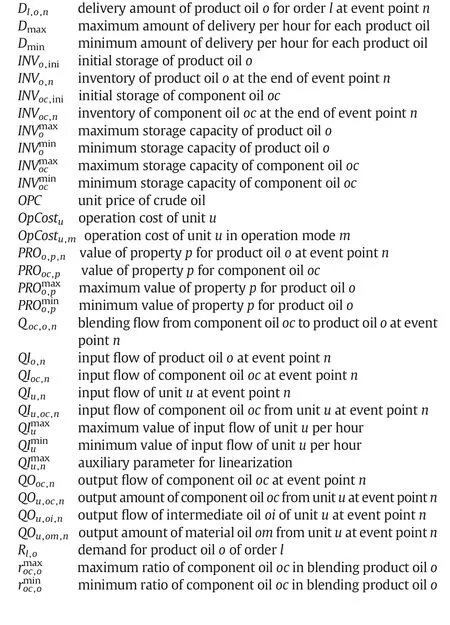
Subscripts

lorder of product oil

moperation mode

nevent point

oproduct oil

occomponent oil for blending

oiintermediate oil

ommaterial oil

pproperty of product oil

uproduction unit

Appendix A.Yields and operation costs of processing units

Operation costs are given in kilograms of oil equivalent per ton;1 kgoe=4.1868×104kJ.

Table 13Statistics of continuous-time and discrete-time models for case 3

Table 14Solutions of continuous-time and discrete-time models for case 3

Table A1Yields and operation costs of ATM and VDU

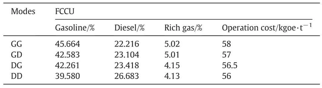
Table A2Yields and operation costs of FCCU

Table A3Yields and operation costs of HDS and ETH

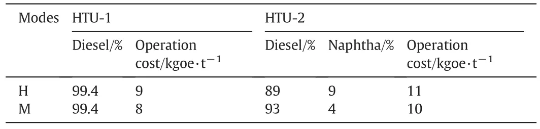
Table A4Yields and operation costs of HTU-1 and HTU-2

Table A5Yields and operation costs of RF and MTBE

Appendix B.Key component concentration ranges of product oils

Table B1Requirements for property of gasoline

Table B2Requirements for property of diesel

Appendix C.Parameters of scheduling model in case study

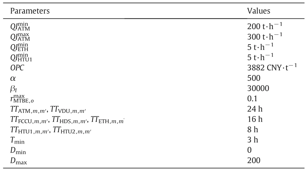
Table C1Parameters of the scheduling model

[1]M.G.Ierapetritou,C.A.Floudas,Effective continuous-time formulation for shortterm scheduling:1.Multipurpose batch processes,Ind.Eng.Chem.Res.37(1998)4341-4359.

[2]M.G.Ierapetritou,C.A.Floudas,Effective continuous-time formulation for shortterm scheduling:2.Continuous and semi-continuous processes,Ind.Eng.Chem.Res.37(1998)4360-4374.

[3]J.M.Pinto,M.Joly,L.Moro,Planning and scheduling models for re finery operations,Comput.Chem.Eng.24(9-10)(2000)2259-2276.

[4]P.M.Castro,A.P.Barbosa-Povoa,H.A.Matos,A.Q.Novais,Simple continuous-time formulation for short-term scheduling of batch and continuous processes,Ind.Eng.Chem.Res.43(1)(2004)105-118.

[5]Z.Jia,M.Ierapetritou,efficient short-term scheduling of re finery operations based on a continuous time formulation,Comput.Chem.Eng.28(6-7)(2004)1001-1019.

[6]P.M.Castro,I.E.Grossmann,New continuous-time MILP model for the shortterm scheduling of multistage batch plants,Ind.Eng.Chem.Res.44(2005)9175-9190.

[7]S.Mouret,I.E.Grossmann,P.Pestiaux,A novel priority-slot based continuous-time formulation for crude-oil scheduling problems,Ind.Eng.Chem.Res.48(2009)8515-8528.

[8]N.K.Shah,M.Ierapetritou,Short-term scheduling of a large-scale oil-re finery operations:Incorporating logistics details,AICHE J.57(2011)1570-1584.

[9]C.A.Floudas,X.Lin,Continuous-time versus discrete-time approaches for scheduling of chemical processes:A review,Comput.Chem.Eng.28(2004)2109-2129.

[10]M.Pan,X.Li,Y.Qian,Continuous-time approaches for short-term scheduling of network batch processes:Small-scale and medium-scale problems,Chem.Eng.Res.Des.87(2009)1037-1058.

[11]I.Harjunkoski,C.T.Maravelias,P.Bongers,P.M.Castro,S.Engell,I.E.Grossmann,J.Hooker,C.Mendez,G.Sand,J.Wassick,Scope for industrial applications of production scheduling models and solution methods,Comput.Chem.Eng.62(2014)161-193.

[12]A.D.Dimitriadis,N.Shah,C.C.Pantelides,efficient modelling of partial resource equivalence in resource-task networks,Comput.Chem.Eng.22(1998)S563-S570.

[13]R.M.Lima,I.E.Grossmann,Y.Jiao,Long-term scheduling of a single-unit multiproduct continuous process to manufacture high performance glass,Comput.Chem.Eng.35(3)(2011)554-574.

[14]S.Mitra,I.E.Grossmann,J.M.Pinto,N.Arora,Optimal production planning under time-sensitive electricity prices for continuous power-intensive processes,Comput.Chem.Eng.38(2012)171-184.

[15]W.Lv,Y.Zhu,D.Huang,Y.Jiang,Y.Jin,A new strategy of integrated control and online optimization on high-purity distillation process,Chin.J.Chem.Eng.18(2010)66-79.

[16]L.Shi,Y.Jiang,L.Wang,D.Huang,Re finery production scheduling involving operational transitions ofmode switching under predictive control system,Ind.Eng.Chem.Res.53(2014)8155-8170.

[17]L.Shi,Y.Jiang,L.Wang,D.Huang,efficient Lagrangian decomposition approach for solving re finery production scheduling problems involving operational transitions of mode switching,Ind.Eng.Chem.Res.54(2015)6508-6526.

[18]R.Raman,I.E.Grossmann,Modeling and computational techniques for logic based integer programming,Comput.Chem.Eng.6(3)(1994)466.

[19]F.You,I.E.Grossmann,Integrated multi-echelon supply chain design with inventories under uncertainty:MINLP models,computational strategies,AICHE J.56(2010)419-440.

[20]X.Hou,Chinese re finery technology,China Petrochemical Press,Beijing,1991 570.

[21]P.M.Castro,I.E.Grossmann,Global optimal scheduling of crude oil blending operations with RTN continuous-time and multi parametric disaggregation,Ind.Eng.Chem.Res.53(39)(2014)15127-15145.