A soft sensor for industrial melt index prediction based on evolutionary extreme learning machine☆

Miao Zhang ,Xinggao Liu ,*,Zeyin Zhang

1 State Key Laboratory of Industrial Control Technology,Department of Control Science and Engineering,Zhejiang University,Hangzhou 310027,China

2 Department of Mathematics,Zhejiang University,Hangzhou 310027,China

1.Introduction

The advanced monitoring and control of polymerization processes,in particular the properties of polymer products,is of major strategic importance to the polymer manufacturing industry.The melt index(MI)of polypropylene is one of the most significant parameters determining different grades of the product.The measurements of the MI are used to control the process operating conditions to meet a desired quality of the intermediate or final products.However,MI is usually evaluated off-line with an analytical procedure in the laboratory,which takes almost 2-4 h[1].The lack of sufficiently fast measurement limits the achievable control performance for polymer quality control.Basically two types of models are considered in literature for MI prediction:mechanism models which use the chemical and physical relationships of variables and statistical models which take advantage of historical observation data.Mogilicharlaet al.[2],Kim and Yeo[3]and Chenet al.[4]developed mechanism models based on process energy and mass balance.But the development of inferential models with the mechanism of polymerization[5-9]is greatly challenged because of the engineering activity and the relatively high complexity of the kinetic behavior and operation of the polymer plants.

One alternative to the mechanism model is the machine learning(or statistical model)that is now being experimented in a wide variety ofindustrialMIprediction applications.The statisticalmodels utilize,assimilate and ‘learn’from the evidence of past MI trends using observational dataset to predict the future.Many types of machine learning algorithmshave recently been proposed in literature such asneuralnetworks(NNs),support vector machines(SVM)and fuzzy logic[10-14].Hanetal.[15]developed three softsensormodels involving SVM,partial least squares(PLS)and artificial NN to predict MI for styrene-acrylonitrile and polypropylene process.Zhangetal.[16]presented sequentially trained bootstrap aggregated NNs for MI estimation.Gonzagaet al.[17]proposed a soft-sensor based on a feed forward artificial NN for real time process monitoring and control of an industrial polymerization process.Furthermore,Shi and Liu[18]compared the performance of the standard SVM,the LSSVM,and the weighted least squares support vector machines(WLSSVM)models.Jianget al.[19]developed a new MI prediction sensor by introducing relevance vector machine(RVM)optimized by Modified particle swarm optimization(PSO)algorithm.Recently a soft sensor based on adaptive fuzzy neural network(FNN)and support vector regression was presented by Zhang and Liu[20].Ahmedet al.[21]proposed a statistical data modeling based on PLS for MI prediction in high density polyethylene processes(HDPE)to achieve energy-saving operation.Zhanget al.[22]proposed a soft sensor based on aggregated RBF neural networks trained with chaotic theory.Despite improvements in the performance of statistical MI prediction models,the development of better predictive models for industrial MI estimation is still an appealing problem.

Extreme learning machine(ELM)developed by Huangetal.is a novel fast machine learning algorithm for single-hidden-layer feedforward neural network(SLFN)[23].In ELM,the weights between input layer and hidden layer are chosen randomly while the weights between hidden layer and output layer are obtained by solving a system of linear matrix equations.Compared with traditional NNs and SVM,ELM offers significant advantages such as fast learning speed,ease of implementation,and minimal human intervention[24,25].Due to its remarkable generalization performance and implementation efficiency,the ELM model has been widely used for the solution of estimation problems in different fields[26-28].Up to now,little information on ELM applications in MI prediction of polypropylene processes has been reported in the literature.In this work,the ELM is therefore explored to predict the MIaccording to a group ofprocess variables in propylene polymerization that can be easily obtained.

However,it is found that ELM may yield unstable performance because of the random assignments of input weights and hidden biases[29].Therefore,an optimization of the ELM structure is essential to improve the performance of the ELM model in the MI prediction.This paper developed a Modified gravitational search algorithm(MGSA)to look for the optimal set of input weights and hidden biases.The MGSA is a swarm-based optimization algorithm which embodies interesting concepts and fully incorporates the social essence of adaptive PSO(APSO)with the motion mechanism of GSA.It adopts co-evolutionary technique to simultaneously update particle positions with APSO velocity and GSA acceleration.Thus,an efficientbalance between exploration and exploitation in the MGSA can be effectively improved.Finally,the newly MI prediction model named MGSA-ELM for propylene polymerization process is achieved.The performance of the proposed models is illustrated and evaluated based on some real industrial processing data.

The rest of the paper is structured as follows:Section 2 provides the theoretic descriptions of the ELM,the MGSA and the proposed evolutionary ELM prediction model.Section 3 and Section 4 present the case study of the paper,where the performance of the proposed approach is evaluated and discussed.Finally Section 5 closes the paper with some concluding remarks.

2.Methodology

2.1.Basic extreme learning machine

Usually an ELM means a three layer neural network[23]in which the weights between input layer and hidden layer are randomly selected and the weights between hidden layer and output layer are determined by solving a generalized system of linear equations(i.e.,by computing the pseudo inverse of a matrix).Fig.1 depicts the basic schematic topological structure of an ELM network.

For a training set ofNsamples(xi,ti),the output of a standard SLFN withnhidden neurons and activation functiong(x)is

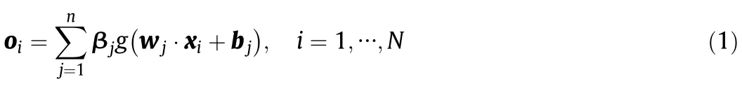
where xiis the inputvector,tiis the outputvector,wjis the inputweight vector,bjis the hidden bias vector,βjis the output weight vector and oiis the actual network output.The aboveNequations can be written compactly as O=Hβ,where

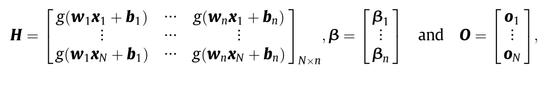
Fig.1.Structure of an ELM network.

H is called the hidden layer output matrix of the neural network.Based on ELM theories,the input weights wjand hidden biases bjcan be randomly assigned instead of tuning.To minimize the cost function‖O-T‖,where T=[t1,t2,…,tN]Tis the target value matrix,the output weights are derived by finding the least square solutions to the linear system Hβ=T,which is given by

where H†is the Moore-Penrose(MP)generalized inverse of the hidden layer output matrix H.

2.2.Modified gravitational search algorithm

2.2.1.Basic GSA

GSA, firstly introduced by Rashediet al.[30],is a population-based meta-heuristic method inspired by the law of gravity and mass interactions.Suppose a system withNPagents in which the position of the agentiis de fined asfori=1,2,… ,NP,whereDis the dimension of the search space.Perform the fitness evaluation for all agents attiteration and also calculate thebestandworstfitness for minimization problem,which are de fined as follows:

wherefiti(t)represents the fitness value of the agentiat iterationt.

Then the gravitational and inertial masses are calculated by the following equations:

The force acting on agentifrom agentjis de fined in Eq.(8)and the total force that acts on agentiis de fined in Eq.(9).

whereMaj(t)is the active gravitational mass related to agentj,Mpi(t)is the passive gravitational mass related to agenti,ε is a small constant,Rij(t)is the Euclidian distance between two agentsiandjin the search space,randjis a random number in the interval[0,1],Kbestis the set of firstKagents with the best fitness values and the biggest masses,andG(t)is the gravitational constant calculated by

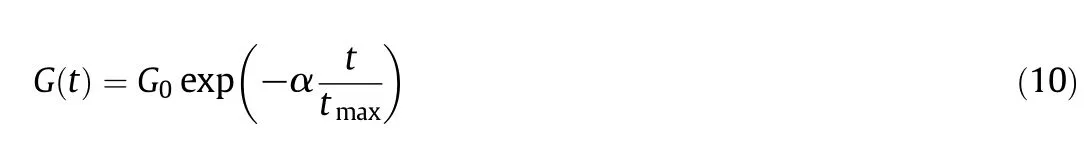
where α is the descending coefficient,G0is the initial gravitational constant,andtmaxis the maximum iteration.

By the law of motion,the acceleration of the agentiwith the inertial massMiiis given by

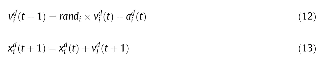
The next velocity of an agentis considered as a fraction of its current velocity added to its acceleration.Therefore,the velocity and position of the agent are calculated as follows:

2.2.2.PSO algorithm

PSO is a biologically inspired computational stochastic search method introduced by Kennedy[31].By randomly initializing the population of particles in the search space,each particle in PSO has a randomized velocity associated to it,which moves through the space of the problem.

In the original PSO,the velocity and position of each particle are updated as follows:

In the adaptive PSO(APSO)algorithm,the acceleration coefficientsc1andc2vary adaptively with each generation[32].The velocity and position of each particle are updated as follows:

wherewis the inertial factor which decreases gradually,kanditermaxare the number of current generation and the maximum number of generations,respectively,c1i,c1f,c2iandc2fare constants.c1decreases from 2.5 to 0.5 andc2increases from 0.5 to 2.5.The APSO is more effective than the original PSO as the search space reduces step by step.

2.2.3.Hybridization of GSA and APSO

In APSO,the exploration ability has been implemented usingpbestand the exploitation ability has been implemented usinggbest[32,33].In GSA,by choosing suitable values for the random parameters(G0andα),the exploration can be guaranteed and slow movementofheavier agents can guarantee the exploitation ability[30,34,35].However,APSO has an aptitude for exploring in a multi-dimensional space while GSA's potentialities are its local exploitation capability.PSO and GSA have supplementary potentialities.

On the other hand,GSA becomes sluggish due to the presence of heavier agents at the end of run.It takes more time to reach the optimal solution.So when allagents of GSA are near a good solution and moving very slowly,gbestin APSO can be considered to help them exploit the global best.Each agent can observe the best solution(gbest)and tend toward it.Moreover,by adjusting the acceleration coefficients of APSO,the abilities of global searching and local searching can be balanced.

Based on the above analysis,the paper hybridizes APSO and GSA by means of applying co-evolutionary technique,treating any particle in the swarm as a particle introduced by GSA.A novel hybrid algorithm,namely Modified GSA(MGSA),is proposed by combining the ability for social thinking in APSO with the local search capability of GSA.The velocity updating formulation in MGSA includes the cooperative contribution of APSO velocity and GSA acceleration and is given below

whereVi(t)is the velocity of particleiat iterationt,ai(t)is the acceleration of particleiat iterationt,gbestis the best solution so far,c1andc2are adaptive acceleration coefficients given by Eqs.(19),(20),wis the inertial factor calculated by Eq.(18),andri1andri2are two random variables in the range[0,1].

In each iteration,the positions of particles are updated as follows:

In MGSA,at first,all particles are randomly initialized,and each particle is considered as a candidate solution.Then,the gravitational constant,inertia factor and adaptive acceleration coefficients are calculated.After evaluating the fitness of each particle,the best and worst fitness values of the population are found.Then,calculate the totalforce and the accelerations for allparticles.After that,the velocities and positions of all particles are updated.The fitness value of each new particle is calculated,and the bestsolution(gbest)and the personalbest position(pbest)so farare also updated.The same iteration steps run circularly to find the optimal solution of the optimization problem,until the maximum iteration number is reached.Note that,whenever the position of a new particle goes beyond its lower or upper bound,the particle will take the value of its corresponding lower or upper bound.

2.3.The proposed evolutionary ELM prediction model

ELM need not spend much time to tune the input weights and hidden biases of the SLFN by randomly choosing these parameters.However,it is also found that ELM tends to require more hidden neurons than traditional gradient-based learning algorithms as well as result in ill-condition problem due to randomly selecting input weights and hidden biases[29].So ELM may have worse performance in case of non-optimal parameters[36,37].In this paper,the proposed MGSA algorithm is used to find the optimal set of input weights and hidden biases for ELM.Thus,the proposed evolutionary ELM prediction model,named MGSA-ELM,is obtained.The root mean square error(RMSE)is chosen as the fitness function,which is given by

The hybrid learning algorithm takes advantage of the merits of ELM and MGSA.First,MGSA combines the ability of social thinking of APSO with the local search capability of GSA,which allows the learning algorithm to avoid the local minima and converge to the global minimum.Moreover,the optimal parameters from MGSA guarantee that ELM has a smalltraining error.Second,in MGSA-ELM,only the inputweights and hidden biasesare optimized by MGSA,while the outputweights are calculated by the least squares method.The learning process will be accelerated because fewer parameters are estimated.Furthermore,since the output weights are calculated by a least squares method at each iteration,the training error is always at a global minimum with respect to the output weights[38].The robustness of training process is highly improved.

Fig.2.Flow chart of the proposed MGSA-ELM model.

Fig.2 shows the flow chart of the MGSA-ELM model and the whole optimization process.To apply the proposed model in MI prediction problem,the following steps have to be taken:

Step 1 Generate the initial population randomly and each individual consists of a set of inputweights and hidden biases.All components in the individual are within the range[-1,1].Initialize the parametersG0,α,c1f,c1i,c2f,c2i,anditermax,and the population sizeNP.Set the iteration numberk=1.

Step 2 Calculate the gravitational constantGby Eq.(10),the weighting factorwby Eq.(18),and the acceleration coefficientsc1andc2by Eqs.(19),(20).

Step 3 For each particle,the output weights are obtained through calculating the MP inverse by Eq.(2).

Step 4 Evaluate the fitness of each particle using the ELM model according to Eq.(23).

Step 5 Calculate the bestsol ution(gbest)and the personal best position(pbest)for the population by comparing the fitness value.

Step 6 Find the best and worst fitness value of the population by Eqs.(3),(4).

Step 7 For each particle,calculate the gravitational and inertial masses by Eqs.(5)-(7),the totalforce by Eq.(9),and the acceleration by Eq.(11).

Step 8 After calculating the accelerations,update the velocities and positions of all particles by Eqs.(21),(22).Whenever the position of a new particle goes beyond its lower or upper bound,the particle will take the value of its corresponding lower or upper bound.

Step 9 Ifi≤NP,go back to Step 7;else go to Step 10.

Step 10 Take the new candidate solution as the set of input weights and hidden biases to obtain the new prediction results.Then update thegbestaccording to the new fitness.

Step 11 Run Step 2 to Step 10 circularly until the maximum iteration numberitermaxis reached,otherwise proceed to Step 12.

Step 12 Output the best solutiongbestas the optimal set of input weights and hidden biases of the ELM model.Finally,the MGSA-ELM model for MI prediction is established.

3.Case Study

The process considered here is a propylene polymerization process located in a plant in China.A highly simplified schematic diagram of the process is illustrated in Fig.3.The process consists of a chain of reactors in series,the first two continuous stirred-tank reactors(CSTR)and two fluidized-bed reactors(FBR).Hydrogen is fed into each reactor,but the catalyst and propylene are added only to the firstreactor along with the solvent.These liquids and gases supply reactants for the growing polymer particles and provide the heat transfer media.Besides,hydrogen entering along with the streams is used as the molecular-weight control agent to produce various grades of polypropylene.The MI of the PP,which depends on the catalyst properties,reactant composition,and reactor temperature,etc.,can determine different brands of products and different grades of product quality.

To develop an effective model to predict the MI from a group of easy-measured variables,a pool of process information formed by nine process variables(t,p,l,a,f1,f2,f3,f4,f5)was selected according to experience and mechanism to construct the model for MI prediction,wheret,p,l,andastand for the process temperature,pressure,level of liquid,and percentage ofhydrogen in vapor phase in the first CSTR reactor,respectively;f1-f3 are flow rates of three streams of propylene into the reactor,andf4 andf5 are flow rates of catalyst and aid catalyst respectively.To avoid the occurrence of abnormal situations and to improve the quality of the prediction model,a greatnumber of operational data has been taken from the DCS historical recorded in the real plant and filtered first,and these are operational data points of polypropylene products of brand F401.Principal component analysis(PCA)is used to determine the important variables surrounding the process.It has been considered that the average sample time for this real propylene polymerization process is about 2 h.Data from the time records are partitioned into three sets which are classified as training,test and generalization sets with 50 data points for training,20 data points for test and the rest for generalization.It should be noted that the test and training set come from the same,whereas the generation set is from another batch.

Fig.3.General scheme of propylene polymerization.

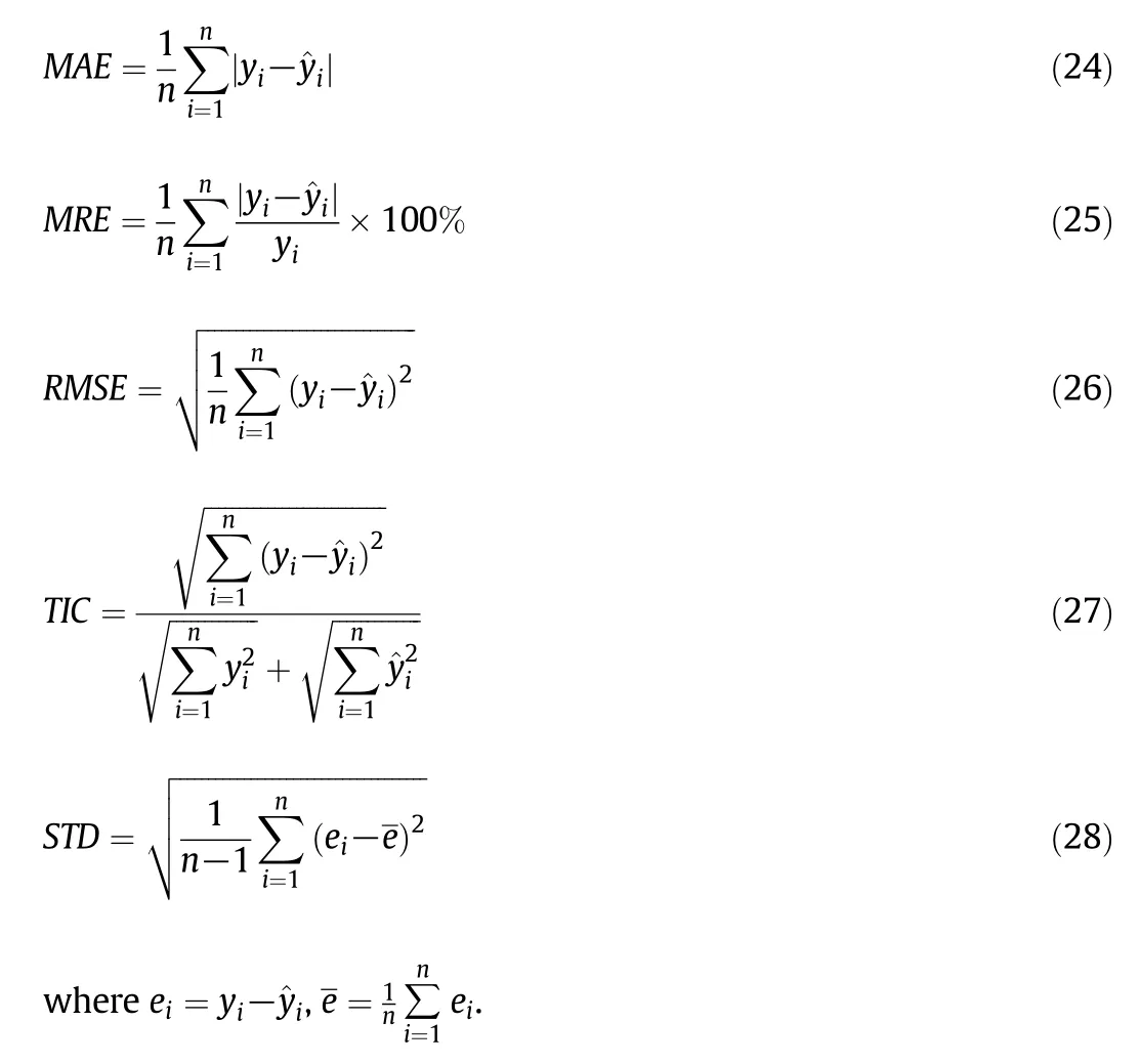
In order to study the prediction accuracy of the proposed model,the difference between the output of the model and the real output is considered and represented in several ways,including mean absolute error(MAE),mean relative error(MRE),root of mean square error(RMSE),Theil's inequality coefficient(TIC)and standard deviation of absolute error(STD)[39].The error indicators are de fined as follows:

4.Results and Discussion

In this research,the parameter settings for the MGSA-ELM are con figured as recommended by the corresponding articles[30,32].The initial gravitational constantG0is set to 100.The descending coefficient αis set to 20.As the acceleration coefficientsc1decreases from 2.5 to 0.5 andc2increases from 0.5 to 2.5,the corresponding constants settings arec1i=0.5,c1f=2.5,c2i=0.5 andc2f=2.5.Besides,the maximum iteration numberitermax=100 and the population sizeNP=50.

In order to investigate the performance of the proposed MGSA-ELM model,several other models,including the ELM,APSO-ELM and GSAELM have also been developed to be as comparison basis.Table 1 lists the performance comparison of different models on the test dataset.Itshows that the MGSA-ELM model has the best performance over all,with anMAEof 0.0180,compared with 0.0335,0.0434 and 0.0775 obtained from the corresponding APSO-ELM,GSA-ELM and ELM models.In terms ofMRE,the MGSA-ELM's prediction accuracy is 0.72%and that of APSO-ELM is 1.31%,much better than ELM(3.26%),error decreasing 77.91%,59.81%respectively.Similar results are observed in terms ofRMSE,with a decrease from 0.0916 to 0.0250.Moreover,theSTDobtained by MGSA-ELM model is 0.0244,while that of APSO-ELM is 0.0475,that of GSA-ELM is 0.0610 and that of ELM is 0.0937.So the MGSA-ELM model has the best stability.It is noted that theTICof MGSA-ELM(0.0049)is quite acceptable when compared with that of APSO-ELM(0.0094),GSA-ELM(0.0118),and ELM(0.0187),which indicates a good level of agreement between the proposed model and the real process.In a word,theMAE,MRE,RMSE,TICandSTDof the MGSA-ELM model are the smallest,with percentage decreases of 76.77%,77.91%,72.71%,73.80%and 73.96%,respectively,compared to the ELM model.The obviously huge percentage decrease further demonstrates the high accuracy of the MGSA-ELM model for the prediction of the MI.

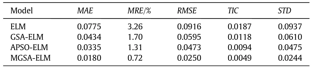
Table 1Performance comparison of different models on the test dataset

Fig.4.Prediction of the optimized models on the test dataset.

Fig.4 illustrates more explicitly in how better the MGSA-ELM model performs than the other models do on the test dataset.As can be seen from the figure,the ELM model marked with crosses shows significant predicting errors,and it is inappropriate to be used in the real industrial plant.The prediction results of the APSO-ELM and GSA-ELM models are better,while the prediction result of the MGSA-ELMmodelmarked with solid squares is the bestand very close to the realMIvalue on mosttesting dataset points.

To specify the universality of the MGSA-ELM model,a comparative study of four models is carried out on the generalization dataset.According to the displayed results in Table 2,the GSA-ELM model and the APSO-ELMmodel have obtained much improved prediction accuracy than the ELM model,but the MGSA-ELM model still has the most accurate prediction results.Compared to the ELM model,the MGSA-ELM model shows a percentage decrease of 55.68%inMREfrom 2.73%to 1.21%.The same happens in terms ofMAE,RMSE,TICandSTD.Moreover,Fig.5 gives an exhibition of how the models perform on the generalization dataset.Obviously,the prediction results of the MGSA-ELM model marked with solid squares are much more accurate than the other models.It proves the excellent university of the MGSA-ELM model for MI prediction both statistically and graphically.

Table 2Performance comparison of different models on the generalization dataset

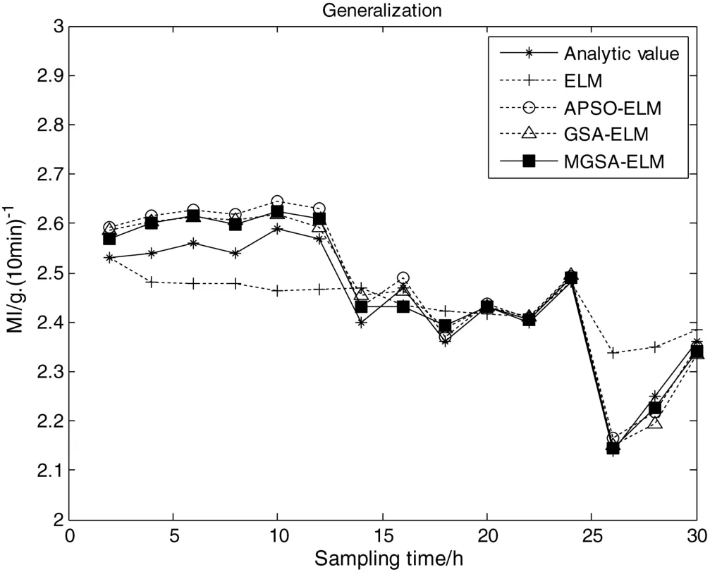
Fig.5.Prediction of the optimized models on the generalization dataset.

Table 3 compares the proposed MGSA-ELM model with other models presented in the open literatures[3,18,21,40].Note that only the research data used in Ref.[18]are the same as that in this paper while the others apply different dataset whose results are for reference only.With the same research data,our work improves the prediction precision fromMRE3.27%presented in Ref.[18]to 0.72%.It shows the advantages of the proposed model.

5.Conclusions

A soft sensor based on an optimized ELMfor PP MI prediction is presented.The ELM is optimized by the MGSA,which hybridizes the APSO and the GSA to choose the optimal set of input weights and hiddenbiases for ELM.According to the comparison results in a real industrial PP plant,the proposed MGSA-ELM model predicts MI with anMREof 0.72%on the test dataset,compared with 1.31%and 1.70%obtained from the APSO-ELM model and the GSA-ELM model.It obtains even smaller prediction error than the ELM model does,with percentage decrease of 77.91%and 55.68%inMREon test dataset and generalization dataset,respectively.Research work shows the effectiveness of the MGSA,and indicates that the proposed MGSA-ELM model is capable of predicting the MI in practical PP industrial processes,and also provides a reference to the soft sensor of other complex industrial processes.Since user-friendly and publicly accessible web-servers represent the future direction for developing practically more useful predictors[41],we shall make efforts in our future work to provide a web-server for the prediction method presented in this paper.

Table 3The comparison between the current work and the published literatures

[1]S.S.Bafna,A.M.Beall,A design of experiments study on the factors affecting variability in the melt index measurement,J.Appl.Polym.Sci.65(1997)277-288.

[2]A.Mogilicharla,K.Mitra,S.Majumdar,Modeling of propylene polymerization with long chain branching,Chem.Eng.J.246(2014)175-183.

[3]T.Y.Kim,Y.K.Yeo,Development of polyethylene melt index inferential model,Korean J.Chem.Eng.27(2010)1669-1674.

[4]X.Z.Chen,D.P.Shi,X.Gao,Z.H.Luo,A fundamental CFD study of the gas-solid flow if eld in fluidized bed polymerization reactors,Powder Technol.205(2011)276-288.

[5]S.Lucia,T.Finkler,S.Engell,Multi-stage nonlinear model predictive control applied to a semi-batch polymerization reactor under uncertainty,J.Process Control23(2013)1306-1319.

[6]A.Shamiri,M.A.Hussain,F.S.Mjalli,M.S.Shafeeyan,N.Mostou fi,Experimental and modeling analysis of propylene polymerization in a pilot-scale fluidized bed reactor,Ind.Eng.Chem.Res.53(2014)8694-8705.

[7]P.Sarkar,S.K.Gupta,Dynamic simulation of propylene polymerization in continuous flow stirred tank reactors,Polym.Eng.Sci.33(1993)368-374.

[8]W.Meng,J.Li,B.Chen,H.Li,Modeling and simulation of ethylene polymerization in industrial slurry reactor series,Chin.J.Chem.Eng.21(2013)850-859.

[9]A.Shamiri,M.A.Hussain,F.S.Mjalli,N.Mostou fi,S.Hajimolana,Dynamics and predictive control of gas phase propylene polymerization in fluidized bed reactors,Chin.J.Chem.Eng.21(2013)1015-1029.

[10]W.Wang,X.Liu,Melt index prediction by least squares support vector machines with an adaptive mutation fruit fly optimization algorithm,Chemometr.Intell.Lab.Syst.141(2015)79-87.

[11]J.Li,X.Liu,H.Jiang,Y.Xiao,Melt index prediction by adaptively aggregated RBF neural networks trained with novel ACO algorithm,J.Appl.Polym.Sci.125(2012)943-951.

[12]N.M.Ramli,M.Hussain,B.M.Jan,B.Abdullah,Composition prediction of a debutanizer column using equation based artificial neural network model,Neurocomputing131(2014)59-76.

[13]L.Ye,H.Yang,A multi-model approach for soft sensor development based on feature extraction using weighted kernel Fisher criterion,Chin.J.Chem.Eng.22(2014)146-152.

[14]Z.Cong,Y.Hao,Consistency and asymptotic property of a weighted least squares method for networked control systems,Chin.J.Chem.Eng.22(2014)754-761.

[15]I.S.Han,C.Han,C.B.Chung,Meltindex modeling with supportvectormachines,partial least squares,and artificial neural networks,J.Appl.Polym.Sci.95(2005)967-974.

[16]J.Zhang,Q.B.Jin,Y.M.Xu,Inferential estimation of polymer melt index using sequentially trained bootstrap aggregated neural networks,Chem.Eng.Technol.29(2006)442-448.

[17]J.Gonzaga,L.Meleiro,C.Kiang,R.Maciel Filho,ANN-based soft-sensor for real-time process monitoring and control of an industrial polymerization process,Comput.Chem.Eng.33(2009)43-49.

[18]J.Shi,X.Liu,Melt index prediction by weighted least squares support vector machines,J.Appl.Polym.Sci.101(2006)285-289.

[19]H.Jiang,Y.Xiao,J.Li,X.Liu,Prediction of the melt index based on the relevance vector machine with Modified particle swarm optimization,Chem.Eng.Technol.35(2012)819-826.

[20]M.Zhang,X.Liu,A soft sensor based on adaptive fuzzy neural network and support vector regression for industrial melt index prediction,Chemometr.Intell.Lab.Syst.126(2013)83-90.

[21]F.Ahmed,L.H.Kim,Y.K.Yeo,Statistical data modeling based on partial least squares:Application to melt index predictions in high density polyethylene processes to achieve energy-saving operation,Korean J.Chem.Eng.30(2013)11-19.

[22]Z.Zhang,T.Wang,X.Liu,Melt index prediction by aggregated RBF neural networks trained with chaotic theory,Neurocomputing131(2014)368-376.

[23]G.B.Huang,Q.Y.Zhu,C.K.Siew,Extreme learning machine:Theory and applications,Neurocomputing70(2006)489-501.

[24]G.-B.Huang,An insight into extreme learning machines:Random neurons,random features and kernels,Cogn.Comput.6(2014)376-390.

[25]G.-B.Huang,H.Zhou,X.Ding,R.Zhang,Extreme learning machine for regression and multiclass classification,IEEE Trans.Syst.,Man Cybern.B Cybern.42(2012)513-529.

[26]D.Wang,M.Alhamdoosh,Evolutionary extreme learning machine ensembles with size control,Neurocomputing102(2013)98-110.

[27]R.C.Deo,M.Şahin,Application of the extreme learning machine algorithm for the prediction of monthly Effective Drought Index in eastern Australia,Atmos.Res.153(2015)512-525.

[28]S.Li,P.Wang,L.Goel,Short-term load forecasting by wavelet transform and evolutionary extreme learning machine,Electr.Power Syst.Res.122(2015)96-103.

[29]Q.Y.Zhu,A.K.Qin,P.N.Suganthan,G.B.Huang,Evolutionary extreme learning machine,Pattern Recogn.38(2005)1759-1763.

[30]E.Rashedi,H.Nezamabadi-Pour,S.Saryazdi,GSA:A gravitational search algorithm,Inf.Sci.179(2009)2232-2248.

[31]J.Kennedy,W.M.Spears,Matching algorithms to problems:An experimental test of the particle swarm and some genetic algorithms on the multimodal problem generator,IEEE,New York,1998.

[32]K.Vaisakh,L.R.Srinivas,K.Meah,Genetic evolving ant direction particle swarm optimization algorithm for optimal power flow with non-smooth cost functions and statistical analysis,Appl.Soft Comput.13(2013)4579-4593.

[33]I.C.Trelea,The particle swarm optimization algorithm:Convergence analysis and parameter selection,Inf.Process.Lett.85(2003)317-325.

[34]E.Rashedi,H.Nezamabadi-Pour,S.Saryazdi,BGSA:Binary gravitational search algorithm,Nat.Comput.9(2010)727-745.

[35]E.Rashedi,H.Nezamabadi-Pour,S.Saryazdi,Filter modeling using gravitational search algorithm,Eng.Appl.Artif.Intell.24(2011)117-122.

[36]F.Ding,System identification—New theory and methods,Science Press,Beijing,2013.

[37]F.Ding,System identification—Performances analysis for identification methods,Science Press,Beijing,2014.

[38]S.McLoone,M.D.Brown,G.Irwin,G.Lightbody,A hybrid linear/nonlinear training algorithm for feedforward neural networks,IEEE Trans.Neural Netw.9(1998)669-684.

[39]D.Murray_Smith,Methods for the external validation of continuous system simulation models:A review,Math.Comp.Model.Dyn.4(1998)5-31.

[40]C.Jin,W.Guizeng,X.Bowen,Prediction of polypropylene melt index based on robust and adaptive RBF networks,Control Decis.14(1999)339-343.

[41]K.-C.Chou,H.-B.Shen,Recent advances in developing web-servers for predicting protein attributes,Nat.Sci.1(2009)63-92.