Forest Canopy Flow Analysis Using Turbulence Model with Source/Sink Terms

YANG Hui(杨会)，FU Hai－ming(付海明)

College of Environmental Science and Engineering，Donghua University，Shanghai201620，China

Forest Canopy Flow Analysis Using Turbulence Model with Source/Sink Terms

YANG Hui(杨会)，FU Hai－ming(付海明)*

College of Environmental Science and Engineering，Donghua University，Shanghai201620，China

A com putational fluid dynam ics(CFD)model was presented to simulate wind flow over a forest canopy for analyzing the w ind flow within and above forest canopies．Unlike previous studies on the canopy flow，the effect of canopy contour on the canopy was considered to develop the simulation method into amore general but comp lex case of w ind flow over a forest canopy，using cedrus deodara and cinnamomum camphora．The desire of this work ismainlymotivated to provide a rationalway for predicting the wind flow within and above vegetation canopies．The model of canopy is not incorporated in the geometricalmodel，and it uses a porous domain combined with k-εtwo-equation turbulence model with source/sink term s．The objectives of this paper are to analyze the contour of pressure and velocity and com pare the simulation results with other works and field measurements．Results are encouraging，as themodel profiles ofmean velocity(u)qualitatively agree wellwith other works com pared with and quantitatively have sim ilar exp lanations as several authors．In conclusion，it is demonstrated that the adoption turbulence model with source/sink terms for forest canopies is proved to be a physically accurate and numerically robust method．The model and method are recommended for future use in simulating turbulent flows in forest canopies．

k-ε;source/sink terms;mean velocity;forest canopy

Introduction

In most regions of the world，w indbreaks are vital in specialized agriculture and horticulture，and information about the w ind flow within the vegetation canopy is important for meteorological，agricultural and ecological studies.For a long time，the scientific study of forest canopies has been motivated by the research of the turbulence and vegetation wind flow within and above a plant canopy.Though w ind flow predictions are essential to obtain accurate site assessments，there have been only a limited number of experimental studies of w ind flow within and above the vegetation canopy.Shaw etal.［1］obtained measured values of momentum and heat fluxes at each height within a corn canopy;W ilson et al.［2］obtained normalized profiles of mean w ind speed and momentum flux from withincanopy and canopy－top measurements;Gash［3］obtained turbulence intensity and w ind velocity near a forest－health interface;Raupach et al.［4］had measured w ind velocity within a model plant in a w ind tunnel;Denmead and Bradley［5］performed experimental studies for scalar transportation on forest canopies;Irvine et al.［6］measured the w ind velocity and the turbulence intensity from a Sitka spruce forest.Duman etal.［7］measured the wind velocity dissipation and turbulent dispersion in atmospheric boundary－layer and canopy flows.Reynolds［8］developed and validated lagrangian probability density function model of horizontally homogeneous turbulencewithin and above plant canopies.Since it is difficult and expensive to perform experiments for measuring airflow within and above forest canopies，for the past several years，various kinds of numerical approaches have been developed as possible solutions to address the experimental problem.However，accurate prediction of w ind flow is difficult due to the complexity in the array of vegetation elements and complex processes of air momentum and eddy diffusion within and above a plant canopy.For a long time the conventional gradient－diffusion theory(K－theory)has been used to study the turbulent air flow within and above the canopy flow.However，calculations based on K－theory don't agree well with field experimental data.A nonlocal closure method for modeling turbulent air flow in the planetary boundary layer(PBL)，namely transient turbulent theory(T－theory)has been developed by Stull et al．［9－13］and Ni［14］. Zeng and Takahashi［15］predicted the wind flow within and above vegetation canopies by first－order closure model，while Albertson et al.［16］used a large eddy simulation(LES)model to simulate eddymotion for3D canopy flows.The advantage of the second－order closure model is that it solves an actual transport equation forε［17］.Yang et al.［18］and Schlegel et al.［19］offered a detailed view of the recirculation regions，and their sensitivity to leaf area index(LAI)by using LES. Other study［20］puts forward a comprehensive discussion regarding the influence of complex terrain and forest edges on themean and turbulent flow statistics.

1 Methodology

1．1 Governing equations

The Reynolds－averaged Navier－Stokes(RANS)equations in their conservation form and the k-εturbulence model were used for thiswork.Assum ing air asan incompressible，viscous，isothermal and New tonian fluid，the steady state 3D RANS governing equations in Cartesian coordinates and introducing the source terms for the canopy interactions，are given as［21］:

whereρ［kg·m－3］is the air density，uiand uj［m·s－1］are the air velocity components，xiand xjare the Cartesian coordinate，p［Pa］is the pressure，μt［kg·m－1·s－1］is the turbulent viscosity，and Su［kg·m－2·s－2］is themomentum source term.is the turbulent Reynolds stress tensor which is modeled by adopting the extended Boussinesq hypothesis［22］，which relates the turbulent stresses to the mean rate of deformation.

where k［m2·s－2］is the mean turbulent kinetic energy，and δijis the Kronecker delta(δij=1 if i=j，andδij=0 if i≠j).Turbulent viscosityμtcan be defined using the turbulent kinetic energy k and the turbulent kinetic energy dissipation rateε:

Here Cμis a constantwith k andεgiven as:

where lmis them ixing length.Then k andεfrom the standard model aremodelled as［23］:

where Sk［m2·s－3］and Sε［m2·s－4］are the source terms for the k andεequations.The production of kinetic energy，Pk［m2·s－3］is given by

Neglecting viscous drag relative to form drag，the canopy momentum source，Suin Eq.(2)is then given by［24］

where Cdis the dimensionless drag coefficient，A is the leaf area density，and U is the average velocity.

Skand Sεare source terms representative of the turbulence generation due to breakage of the mean－flow motion of the vegetation elements［25］:

whereβp(∈［0，1］)is the fraction of the mean flow kinetic energy converted to wake－generated k by canopy drag，andβdhas less physicalmeaning but is considered as the fraction of k dissipated by interactions with the vegetation.The constant Cε4in the Sεmodel is justified by mixing length anisotropy［24］. Table 1 presents a summary of all the contants of the stand k-ε turbulencemodel.

Table 1 Constants of standard k-εturbulentmodel

1．2 Simulation cases

The whole cedrus deodara and cinnamomum camphora field are included in simulations.The boundary conditions considered for the simulations are shown in Fig.1.Air is assumed to flow into the simulation domain through a velocityinlet，the inlet horizontal velocity profiles is defined as u(z)=δ0(110m)is the boundary layer depth and leaves it from a pressure－outlet boundary condition.At the ground surface non－slip boundary conditions togetherwith standard wall functions were applied as described by Launder and Spalding［23］.A slip boundary condition was assigned to the lateral sides and the domain top.The inlet and outlet boundary conditions are placed at a distance of 5 times the canopy diameter along the x axis in upstream，and 5 times the canopy diameter downstream from the canopy，3 times the canopy diameter along the y axis and 3 times the average height of the tree along the z axis.As can be seen from Fig.1，we have used periodic boundary conditions on the sides of the computational box.Nevertheless，choice of the lateral boundary conditions does notaffect the simulation results as the flow ismainly in the through－plane direction.

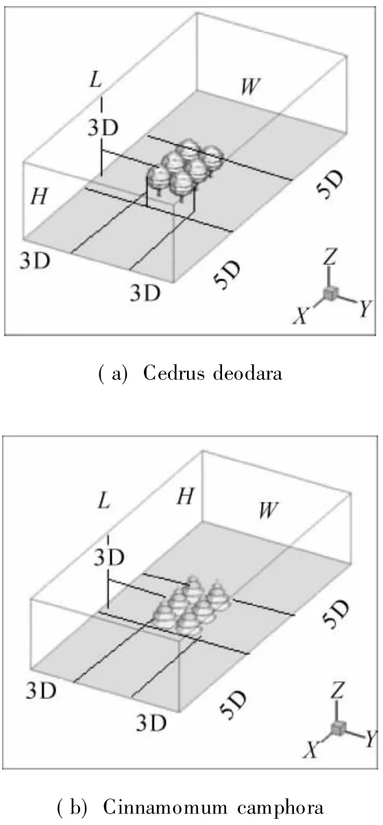
Fig.1 Simulation domain for simulating the effects of trees and direction

2 Results and Discussion

This section puts forward a comparison between the experimental measurements and the computational fluid dynam ics(CFD)simulations.Wind velocity results are presented as the ratio of the predicted velocity over the friction velocity u*.The friction velocity u*is evaluated using a reference velocity，and the velocity and the reference height were imposed at the top of the domain(utop)and the height of the domain(Ztop)，respectively:

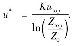
where K=0.42 is the dimensionless von kármán constant，andis aerodynam ic roughness length(1.28×10－2m).Here，=1.03 m/s.

2．1 Velocity and pressure fields

Bothmethods show that the flow deviates around the tree. In the wake behind the trees，the velocity is significantly reduced.Velocity contour plots in Fig.2，while pressure contours plots in Fig.3.The plots are taken on a plane at the center of a canopy domain and a plane between two canopy domains along the directions of flows of cedrus deodara and cinnamomum camphora，respectively.

Figures 2 and 3 show velocity contours and pressure contours，respectively.Along the simulation domain on the xzplane that passes through the centre of a canopy(y/W=0.7) and the centre between two canopy(y/W=0.5)，show ing detail airflow conditions upstream and downstream of the flow of cedrus deodara and cinnamomum camphora，respectively.It illustrates to what extent the two models represent the wake velocity.

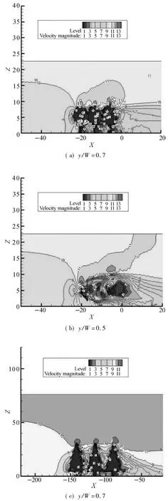
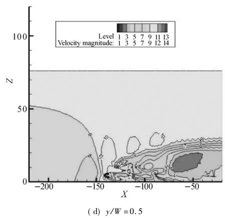
Fig.2 Velocity contours along the simulation domain on the xz planewith inlet velocity u=10 m/s:(a)＆(b)cedrus deodara;(c)＆(d)cinnamomum camphora

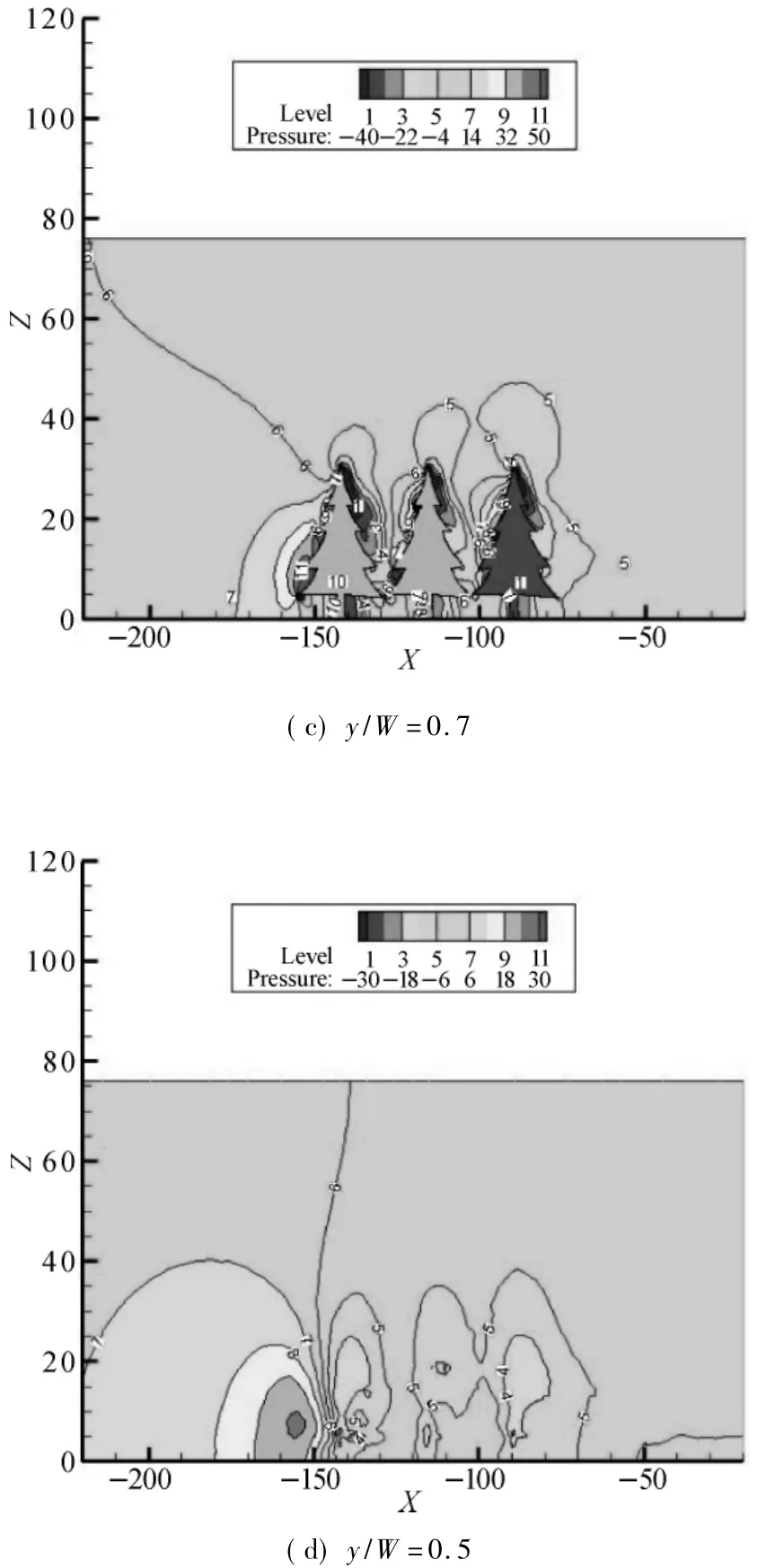
Fig.3 Pressure contoursalong the simulation domain on the xz plane with inlet velocity u=10 m/s:(a)＆(b)cedrus deodara; (c)＆(d)cinnamomum camphora

Due to a blocking e ffect(the air flow is slowing down inside the forest region due to the effects of leaf and branch drag on air flow)，strong velocity gradient and pressure gradient can be created，also the blocking can lead to the formation of long recirculative regions(wakes)［26］.According to these plots，both the two planes of the velocity at the wake，the average velocity in thewake exhibits an irregular non－symmetric contour pattern.Obviously，themean w ind speed reaches its peak just above the plant canopy，while the static pressure reaches its peak once reaches the vegetation region.

Figures 4(a)－(b)and(c)－(d)compare the mean velocity u and the static pressure calculated by the k－εtwoequation turbulentmodel with source/sink terms，respectively，with height z/h=1/2.The horizontal velocity passes through the centre between two canopies along the z/h=0.5(Figs.4 (a)and(b))line shows a slight decrease from the fully developed state up to the edge of the vegetation at x/h=－4 and－7 positions for cedrus deodara and cinnamomum camphora，respectively.Then，the air flow accelerates，and strong suppression of themean w ind speed takes place after reaching its second peak at x/h=3.5 and 5 positions，respectively，while the horizontal velocity passing through the centre of a canopy exhibits differentbehaviors along the z/h=0.5(Figs.4(a)and (b))line.Here，in contract to the previous location，the second peak inside the forest canopies is not present anymore and themean velocity strongly suppressed along the entire forest region.Moreover，the flow recovery of w ind speed starts earlier at x/h=0 and－2 positions for cedrus deodara and cinnamomum camphora，respectively，in other words，immediately after leaving the forest region.Obviously，the minimum average w ind speed occurs in the middle of the canopy，where the turbulence intensity reaches its maximum，and rapidly recovery further to leeward.

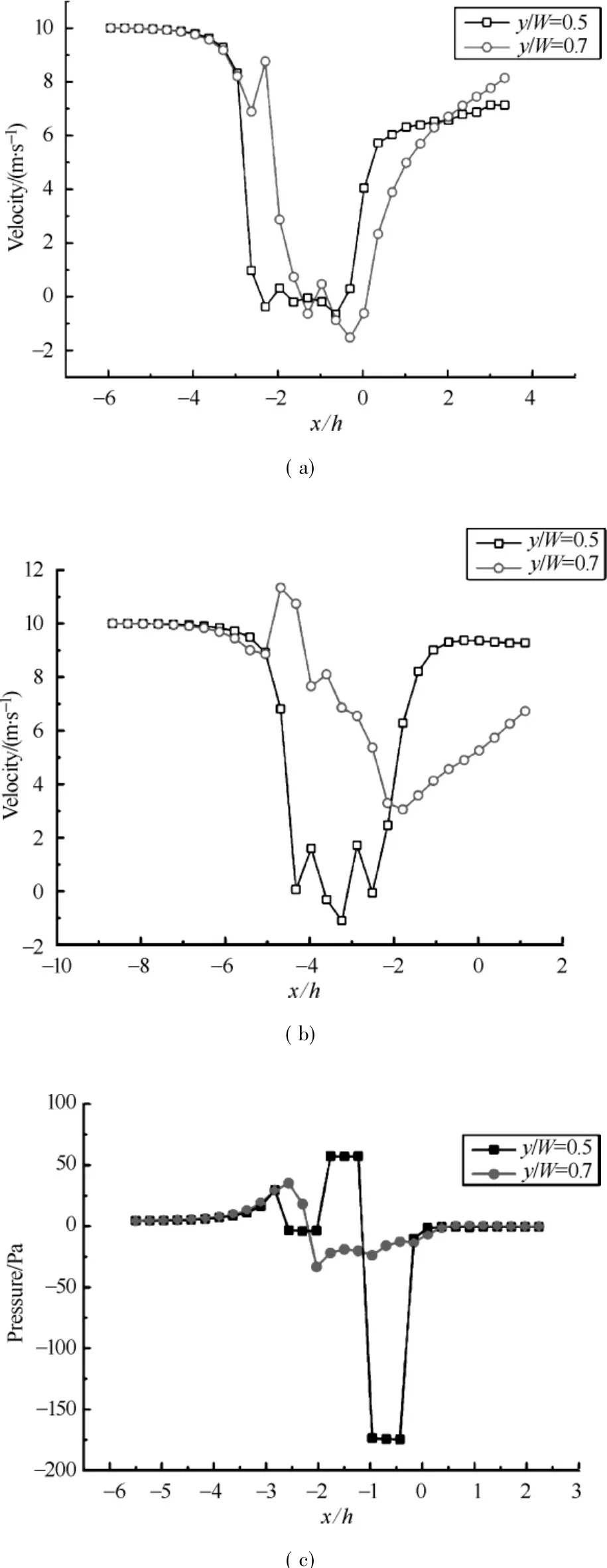
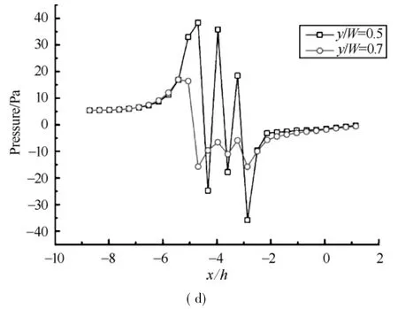
Fig.4 Simulated normalized mean wind speed and pressurewith z/h= 0.5:(a)＆(b)cedrus deodara;(c)＆(d)cinnamomum camphora

2．2 Profiles of mean air velocities

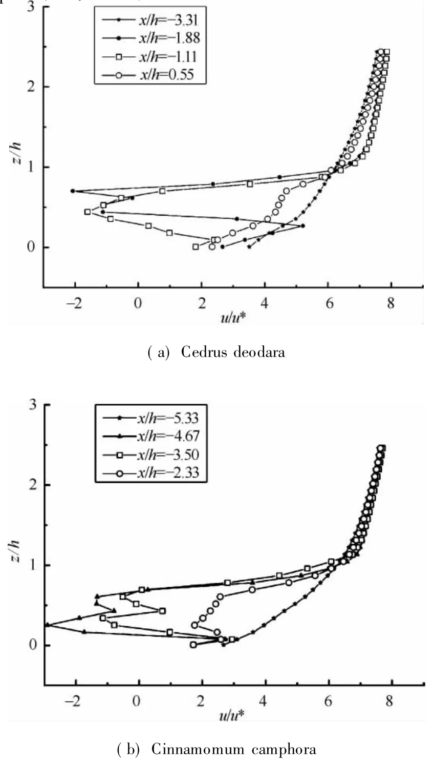
Fig.5 Normalized vertical profiles of average longitudinal air velocity (u)obtained by simulations from(a)cedrus deodara and(b) cinnamomum camphora respectively with y/W=0.5

Figures 5(a)and(b)compare the mean velocity u calculated by the k－εtwo－equation turbulent model with source/sink terms at different characteristic locations:x/h=－3.31，－1.88，－1.11，0.55，and x/h=－5.33，－4.67，－3.50，－2.33 for cedrus deodara and cinnamomum camphora，respectively.Four characteristic locations show detail airflow conditions upstream and downstream of the flow of cedrus deodara and cinnamomum camphora，respectively.The horizontal velocity passes through the centre of vegetation canopies along the y/W=0.5(Figs.5(a)and(b))line shows a decrease from the fully developed state up to the edge of the vegetation canopy at z/h=0.5 location for cedrus deodara and cinnamomum camphora，respectively.Then，the air flow accelerates，and strong suppression of the mean w ind speed takes place after reaching its nadir at about z/h=0.5 for both cedrus deodara and cinnamomum camphora.And the peak of air mean velocity occurs when z/h reaches about 2.Furthermore，the horizontal velocity exhibits different behaviors upstream of the flow，the mean velocity slightly accelerates along entire z axis，and the airmean velocity reaches its peak at about z/h= 2.

Normalized vertical profiles of average longitudinal air velocity(u)obtained by simulation using the 3D canopies in the domain with source/sink terms in a porous domain are compared with other works and field measurements from Raupach et al.［4］，Albertson et al.［16］，Duman et al.［7］，and Reynolds［8］in Fig.6.And u is normalized with the friction velocity(u*)and the vertical axis(z)is normalized with the average tree height h.The comparison of the simulated mean w ind speed profile with the experimental results from literature shows that there is reasonable agreement for the use of twoequation turbulentmodelwith source/sink terms.

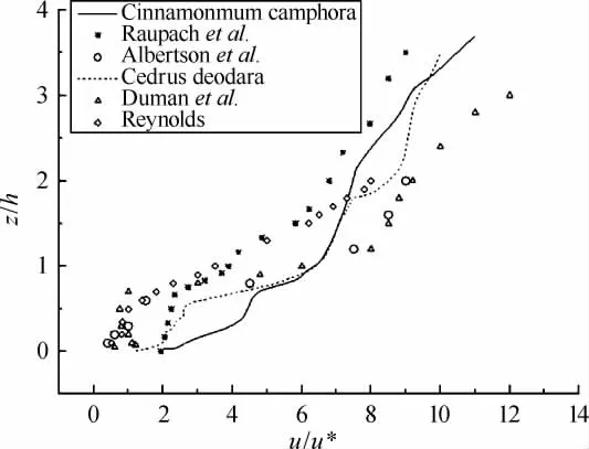
Fig.6 Normalized vertical profiles between average longitudinal air velocity(u)obtained by simulation and otherworks

3 Conclusions

Bymodeling the3D structure of the forest canopy using 2D canopy geometry in which the vegetation is packed in square and circle configurations，itprovides the basis ofmostexsiting forest canopy simulation model that has been developed over the past 50 years.In the paper，3D canopy architectures with similar canopy contour configuration as cedrus deodara and cinnamomum camphora are introduced to predict pressure drop and mean velocity profile.In addition，the inlet horizontal velocity profiles is introduced as u(z)andδ0(110 m)is the boundary layer depth，which are different from the previous studies.

For turbulent air flow within and above the vegetation canopy，strong turbulent shear takes place within and above the plant canopy due to the effects of leaf and branch drag on air flow.The model profiles of mean velocity(u)qualitatively agree well with other works compared with and quantitatively have similar explanations.A comparison of results from simulated velocity profile and fieldmeasurements shows that the two－equation turbulent model with source/sink terms can wellpredict the wind speed profile within and above the forest canopies.

However，the mean velocity and static pressure data are lim ited in this paper，and the presented integrated CFD modelling approach will be validated in the further experiments. At the same time，the turbulent kinetic energy k，the turbulent kinetic energy dissipation rateεand the turbulent intensity have not been analyzed and validated.So，in subsequentworks，the shortages showed above will be studied.

［1］Shaw R H，Silversides R H，ThurtellGW.Some Observations of Turbulence and Turbulent Transport within and above Plant Canopies［J］.Boundary-Layer Meteorol，1974，5(4):429－449.

［2］W ilson J D，Ward D P，Rhurtell G W，et al.Statistics of Atmospheric Turbulence within and above a Corn Canopy［J］. Boundary-Layer Meteorol，1982，24(4):495－519.

［3］Gash JH C.Observations of Turbulence Downw ind of a Forest－Heath Interface［J］.Boundary-Layer Meteorology，1986，36 (3):227－237.

［4］Raupach M R，Coppin P A，Legg B J.Experiments on Scalar Dispersion within a Model Plant Canopy Part I:the Turbulence Structure［J］.Boundary-Layer Meteorology，1986，35(1/2): 21－52.

［5］Denmead O T，Bradley E F.On Scalar Transport in Plant Canopies［J］.Irrigation Science，1987，8(2):131－149.

［6］Irvine M R，Gardiner B A，Hill M K.The Evolution of Turbulence across a Forest Edge［J］.Boundary-Layer Meteorology，1997，84(3):467－496.

［7］Duman T，Katul G G，Siqueira M B，et al.A Velocity－Dissipation Lagrangian Stochastic Model for Turbulent Dispersion in Atmospheric Boundary－Layer and Canopy Flows［J］. Boundary-Layer Meteorology，2014，152(1):1－18.

［8］Reynolds A M.Development and Validation of a Lagrangian Probability Density Function Model of Horizontally－Homogeneous Turbulence within and above Plant Canopies［J］.Boundary-Layer Meteorology，2012，142(2):193－205.

［9］Stull R B.Transilient Turbulence Theory.Part I:the Concept of Eddy M ixing across Finite Distances［J］.Journal of the Atmospheric Sciences，1984，41(23):3351－3367.

［11］Stull R B.A Convective Transport Theory for Surface Fluxes［J］.Journal of the Atmospheric Sciences，1994，51(1):3－22.

［12］Stull R B，Hasagswa T.Transilient Turbulence Theory.Part II: Turbulent Adjustment［J］.Journal of the Atmospheric Sciences， 1984，41(23):3368－3379.

［13］Stull R B，Driedonks A G M.Application of the Transilient Turbulence Parameterization to Atmospheric Boundary－Layer Simulations［J］.Boundary-Layer Meteorology，1987，40(3): 209－239.

［14］NiW G.A Coupled Transilience Model for Turbulent Air Flow within Plant Canopies and the Planetary Boundary Layer［J］. Agricultural and Forest Meteorology，1997，86(1/2):77－105.

［15］Zeng P T，Takahashi H.A First－Order Closure Model for the W ind Flow within and above Vegetation Canopies［J］. Agricultural and ForestMeteorology，2000，103(3):301－313.

［16］Albertson J D，Katul G G，Wiberg P.Relative Importance of Local and Regional Controls on Coupled Water，Carbon，and Energy Fluxes［J］.Advances in Water Resources，2001，24(9/ 10):1103－1118.

［17］Siqueira M，Katul G，Tanny J.The Effect of the Screen on the Mass，Momentum，and Energy Exchange Rates of a Uniform Crop Situated in an Extensive Screen House［J］.Boundary-Layer Meteorology，2012，142(3):339－363.

［18］Yang B，Raupach M R，Shaw R H，et al.Large－Eddy Simulation of Turbulent Flow across a Forest Edge.Part I:Flow Statistics［J］.Boundary-Layer Meteorology，2006，120(3): 377－412.

建立建全体制机制是推动全行业创新创业教育改革的重中之重，完善课程体系建设、加强师资队伍建设、保障流畅的市场运营是完善机制正常运行的三大法宝，配合高效成果转化，加强校企合作，设立创新创业孵化基地，多方协同发力，为医学生想创业、能创业提供更好的平台和坚实的保障。

［19］Schlegel F，Stiller J，Bienert A，et al.Large－Eddy Simulation of Inhomogeneous Canopy Flows Using High Resolution Terrestrial Laser Scanning Data［J］.Boundary-Layer Meteorology，2012，142(2):223－243.

［20］Belcher S E，Harman I N，Finnigan J J.The Wind in the willows:Flows in Forest Canopies in Complex Terrain［J］. Annual Review of Fluid Mechanics，2012，44(1):479－504.

［21］Endalew A M，Hertog M，Gebrehiwot M G，et al.Modelling Airflow within Model Plant Canopies Using an Integrated Approach［J］.Computers and Electronics in Agriculture，2009，66(1):9－24.

［22］Versteeg H K，Malalasekera W.An Introduction to Computational Fluid Dynam ics［M］.NJ:Prentice－Hall，Englewood Cliffs，1995:257.

［23］Launder B E，Spalding D B.The Numerical Computation of Turbulent Flows［J］.Computer Methods in Applied Mechanics and Engineering，1974，3(2):269－289.

［24］Sanz C.A Note on k－εModelling of Vegetation Canopy Air－Flows［J］.Boundary-Layer Meteorology，2003，108(1):191－197.

［25］Katul G G，Mahrt L，Poggi D，et al.One－and Two－Equation Models for Canopy Turbulence［J］.Boundary-Layer Meteorology，2004，113(1):81－109.

［26］KenjerešS，ter Kuile B.Modelling and Simulations of Turbulent Flows in Urban Areas with Vegetation［J］.Journal of Wind Engineering and Industrial Aerodynamics，2013，123A:43－55.

X513;S731.2

A

1672－5220(2015)04－0588－06

date:2014－07－29

s:National Natural Science Foundations of China(Nos.51178094，41371445)

*Correspondence should be addressed to FU Hai－m ing，E－mail:fhm@dhu.edu.cn