Automatic estimation and removal of noise on digital image*
Tuananh Nguyen, Beomsu Kim, Mincheol Hong
(School of Information and Telecommunication, Soongsil University, Seoul 156-743, Korea)
Automatic estimation and removal of noise on digital image*
Tuananh Nguyen, Beomsu Kim, Mincheol Hong
(School of Information and Telecommunication, Soongsil University, Seoul 156-743, Korea)
An spatially adaptive noise detection and removal algorithm is proposed. Under the assumption that an observed image and its additive noise have Gaussian distribution, the noise parameters are estimated with local statistics from an observed degraded image, and the parameters are used to define the constraints on the noise detection process. In addition, an adaptive low-pass filter having a variable filter window defined by the constraints on noise detection is used to control the degree of smoothness of the reconstructed image. Experimental results demonstrate the capability of the proposed algorithm.
noise estimation; denoising; noise parameters; local statistics; adaptive filter
0 Introduction
In general, a digital image represents the degraded version of an original image by one or a combination of many sources, such as transmission errors, faulty memory locations and the imaging system[1]. The additive noise raises the performance degradation of many applications, such as video/image coding, object recognition, and so on. Therefore, an adequate denoising method should be used to maximize the performance of the subsequent image/vision applications.
1 Main research work
This section should contain a description of what you have done about your work, what kind of instrumentation and methods that you have used or developed. You should provide detailed information for other researchers to use or repeat your process. If you are using a procedure or instrumentation which has already been published, please include a reference to that paper.
The goal of denoising is to suppress noise while preserving the integrity of edge and detailed information associated with an original image. A number of techniques for doing this have been reported in past years[1-3]. Adaptive median filters have been widely used due to their computational efficiency[4-6], but they lead to overly blurred results. Also, an adaptive bilateral filter (ABF) is presented in Ref.[7], where the intensity value at each pixel is replaced by the weighted average of both the pixel intensity difference and the pixel spatial difference. It has the capability of better preserving a sharper edge than adaptive median filtering methods. However, its performance is limited, since noise detection is not incorporated into the noise removal process.
Over the years, many noise removal algorithms coupled with a noise detector have been used. In Ref.[8], a switching-based adaptive weighted mean (SAWM) filter is presented, where the corrupted and uncorrupted pixels are detected by comparing the difference between a current pixel and its neighbours in four directional windows with a predefined threshold, and then, an adaptive weighted mean filter is applied to the detected noisy pixels. In addition, a noise reduction algorithm with a statistical hypotheses tests (SHT)-based noise detector introduced in Ref.[9] uses sample correlation in different orientations to estimate the noise information. The above methods, by using local information, result in better suppression of additive noise than doing adaptive median/mean filter approaches. However, they still lead to unsatisfactory results, since a reasonable constraint is not derived from the local statistics. Therefore, it is necessary to incorporate prior knowledge about an original image into the denoising process so that the number of local features can be well-reflected on the reconstructed image.
In this paper, we propose a spatially adaptive noise detection and removal algorithm. Under the assumption that an observed image and its additive noise are Gaussian-distributed, noise parameters are estimated using the local statistics of an observed image. Then the parameters are used to define the noise detector, and an adaptive filter is applied to the corrupted pixels. According to the estimated noise parameters and the noise detector, the modified Gaussian filter is used to effectively suppress the additive noise, where different filter window sizes are used to control the degree of smoothness of the reconstructed image. This paper is an enhanced version of Ref.[10]: A more robust noise detector is defined by using the estimated noise, and a variable filter window is used to flexibly control the filter strength for noise removal. In addition, the algorithm is described in more detail.
This paper is organized as follows. In section 2, the proposed denoising algorithm is presented. In order to define constraints for noise detection, the estimation of noise parameters based on local statistics is described. In addition, an adaptive Gaussian filter having different window sizes controlling the degree of smoothness is addressed. Finally, sections 3 and 4 describe the experimental results and a conclusion, respectively.
2 Proposed adaptive denoising algorithm using parameter estimation
When an original image is degraded by signal-independent additive noise, the typical degradation model at point (i,j) in a two-dimensional coordinate can be written as
y(i,j)=x(i,j)+n(i,j),
(1)
where x, y and n represent an original image, the observed degraded image and the additive noise, respectively[1]. For effective denoising, it is desirable to derive a reliable noise detection process that can detect the degree of the noise as well as the position of noise. Many related studies have been presented in past years[8-13]. In this paper, we use local statistics, such as local mean and local variance, to define a noise detection process, under the assumption that an observed image and the additive noise take a Gaussian distribution. In addition, we discuss an adaptive Gaussian filter that has a variable filter window size for controlling the filter’s strength.
2.1 Noise detection by parameter estimation
In general, noise visibility to the human viewer depends on the local statistics[14]. For example, when the same noise is added to low- and high-activity regions, the noise within the low-activity region is more visible than that within the high-activity region. Also, a noise with a brighter background is more visible than that with a darker background. Typically, local activity and brightness can be represented as local variance and a local mean. For pixel f(i,j) of an image, the local weighted mean and standard deviation with a square window of size (2K+1)×(2K+1) can be written as
(2)
(3)
where ω(m,n) denotes the (m,n)-th weighting coefficient and |·| represents the absolute operator. In this paper, we use uniform coefficients, with K=1 such that ω(m,n)=1 for -1≤m, n≤1, due to the computational cost.
In practice, information about noise is very restricted, and therefore a reasonable estimation is desirable to effectively suppress the noise. Noise estimation approaches have appeared in Refs.[12-14]. These approaches can be classified as block-based estimation or pixel-based smoothing estimation in a spatial domain.
In this paper, we present a way to estimate the parameters of the additive noise using the image difference between an observed noisy image and the smoothing image. The smoothing filter can be justified in several ways. In our work, a low-pass filter using Eqs.(2) and (3) is used. For a pixel centred at the (i,j) position with a 3×3 filter window, it can be written as
(4)
In Eq.(4), for -1≤m, n≤1, Z1and L1represent the normalizing constant and a tuning parameter, respectively. The low-pass filter coefficient in Eq.(4) becomes smaller as the local variance becomes higher and the local mean becomes lower. Therefore, the filtered image retains important features around higher-activity regions. On the other hand, the isolated components within flat regions result in over-blurring. Therefore, we consider the difference between the observed image and the filtered image to have characteristics similar to those of the noise. Then, the estimated noise can be written as

(5)
where * is the convolution operator. Then, the local mean and standard deviation of the estimated noise can be obtained by Eqs.(2) and (3). Under the assumption that an observed image having a Gaussian distribution represents the degraded version as signal-independent zero-mean Gaussian distributed noise, information about the estimated original image can be derived as

(6)
It is clear that the observed pixel can be regarded as a corrupted one, if y(i,j) is far away from μK(i,j), under the assumption that the abrupt transition with respect to the neighbouring pixels rarely occurs. On the basis of the above properties, we define a noise detection function as
(7)
where T1and T2eenote thresholds (T2gt;T1). In Eq.(7), the value of the flag represents the degree of the corruption of y(i,j). In general, when the predefined thresholds in Eq.(7) are used, the performance of the noise detection is very sensitive to the degree of the noise or the degree of local activity of an image.
As pointed out, the thresholds should be a function of the additive noise with respect to μK(i,j), under the assumption that an uncorrupted pixel is within a certain range. In addition, the thresholds should become lower as σK(i,j) becomes higher, since σK(i,j) represents the amount of the estimated noise. On the other hand, a smaller σK(i,j) leads to tighter thresholds. This is in agreement with the noise-masking property of the human visual system (HVS)[14]. From the assumption about the noise, the probability density function (PDF) of the observed image can be written as
fy(y)=fx(x)+fn(n).
(8)

(9)
where T1is experimentally determined. Eq.(9) means that tighter thresholds are applied as the estimated noise increases, and that uncorrupted regions (σK(i,j)≈0) lead to looser thresholds, as expected.

Fig.1 Example of determining thresholds of degraded image having a Gaussian propability density function
2.2 Denoising using variable window filter
The problem at hand is to suppress the noise according to noise detection as defined in Eqs.(7) and (8). A Gaussian filter type is an adequate way to handle the noise, since it is represented as a function of the local mean and the local standard deviation. For the denoising problem, edge preservation and noise suppression are both carefully considered. To do this, the local statistics for an original image should be incorporated into the reconstruction process. For example, a weaker low-pass filter is adequate to suppress the noise when the local activity of the estimated original image increases, so that detailed information can be well preserved. In addition, it is reasonable to use a stronger low-pass filter when the background is brighter, since the noise with brighter background is more visible.
The filter satisfying the above conditions can be written as
(10)
In Eq.(10), for -U≤m, n≤U, U denotes a filter window size. In addition, Z2and L2represent the normalizing constant and a constant of the noise removal filter, respectively. Eq.(10) means that the local parameters of the estimated original image are used to control the filter strength.
In addition, the information of the estimated can be used to control the filter strength. The filter strength can be justified in several ways[3].
In this paper, we use a variable-length sliding-window filter to control the filter strength. A strong low-pass filter having a larger filter window is applied to heavily corrupted pixels. On the other hand, a weak low-pass filter with a smaller filter window is used to suppress lightly corrupted ones. Even though a larger filter window is effective for suppressing the noise as the noise becomes more distinguishable, it leads to over-blurred results. Also, small filter windows result in the failure of noise suppression.
In this paper, according to the noise classification in Eq.(7), the window size is defined as
(11)
where the window sizes for each flag value are experimentally determined. The reconstructed image can be obtained in direct, recursive, or iterative ways. In order to minimize the computational cost, direct noise filtering is used. Then, the reconstructed image can be written as
(12)
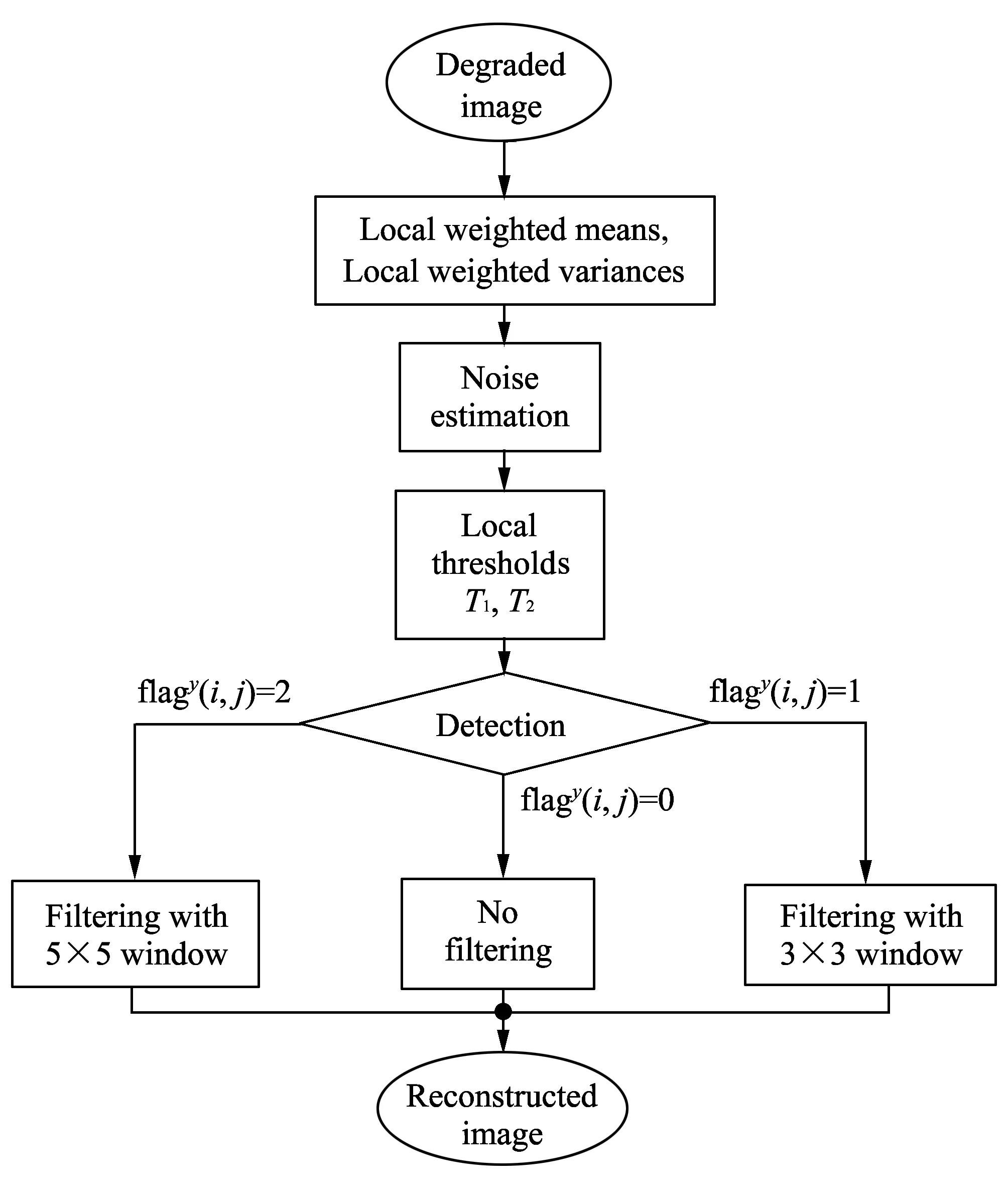
Fig.2 Flow chart of proposed algorithm
The novelty of the proposed algorithm is that it has the capability of adaptively removing the additive noise according to the estimation of noise parameters using local statistics, without knowledge of the original image or noise. Fig.2 shows the entire procedure of the proposed algorithm.
3 Experimental results
Several experiments have been conducted with various images. Gaussian noise with various signal-to-noise ratios (SNRs) was added to the original images. We compared the proposed algorithm with an ABF[7], a statistical hypotheses test based filter (SHTF)[9], and a fast efficient filter (FAEF)[10]. In order to evaluate the performance of the noise detection algorithms, the following noise detection fidelity is used as
(13)
where FP, MPand TPrepresent the number of detection “fault” pixels, the number of detection “missing” pixels, and the number of total pixels in an image. A detection “fault” pixel means an uncorrupted pixel is considered corrupted. On the other hand, a “missing” pixel means a corrupted pixel is detected as uncorrupted. Also, the peak signal-to-noise ratio (PSNR) and structural similarity index (SSIM) used in Ref.[15] a used here to evaluate the performance of the noise removal filter.
In Eq.(4), as the tuning parameter, L1, gets higher, missing detection error gets higher. Furthermore, a smaller value leads to a higher fault detection error. Experiments verified that 0.01≤L1≤0,05 is a good range for minimizing detection error. In addition, as the filter constant, L2, in Eq.(10) grows smaller, a stronger low-pass filter is applied to an observed image, leading to over-smoothing of the reconstructed image. A larger value leads to a weaker low-pass filter, resulting in a failure to minimize the noise. It was observed that 0.01≤L2≤0,05 is a good range for the constant. In this set of experiments, the results obtained with the 256×256-sized “Lena”, “Cameraman” and “Goldhill” images are described.
Tables 1-2 summarize the performance comparisons with respect to DF, PSNR and SSIM.
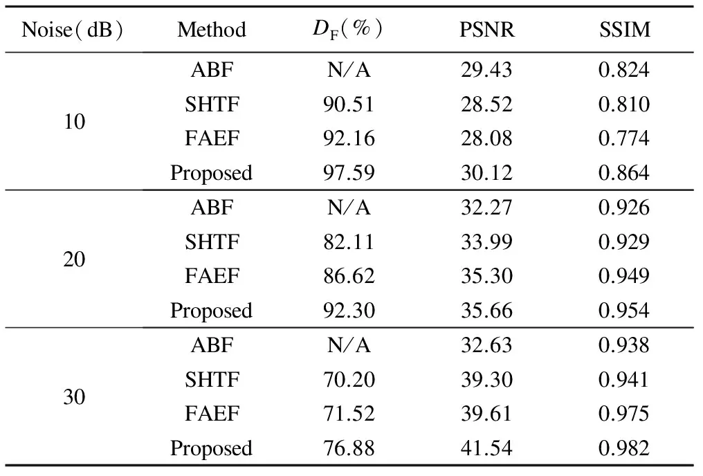
Table 1 Performance comparison with “Lena” image
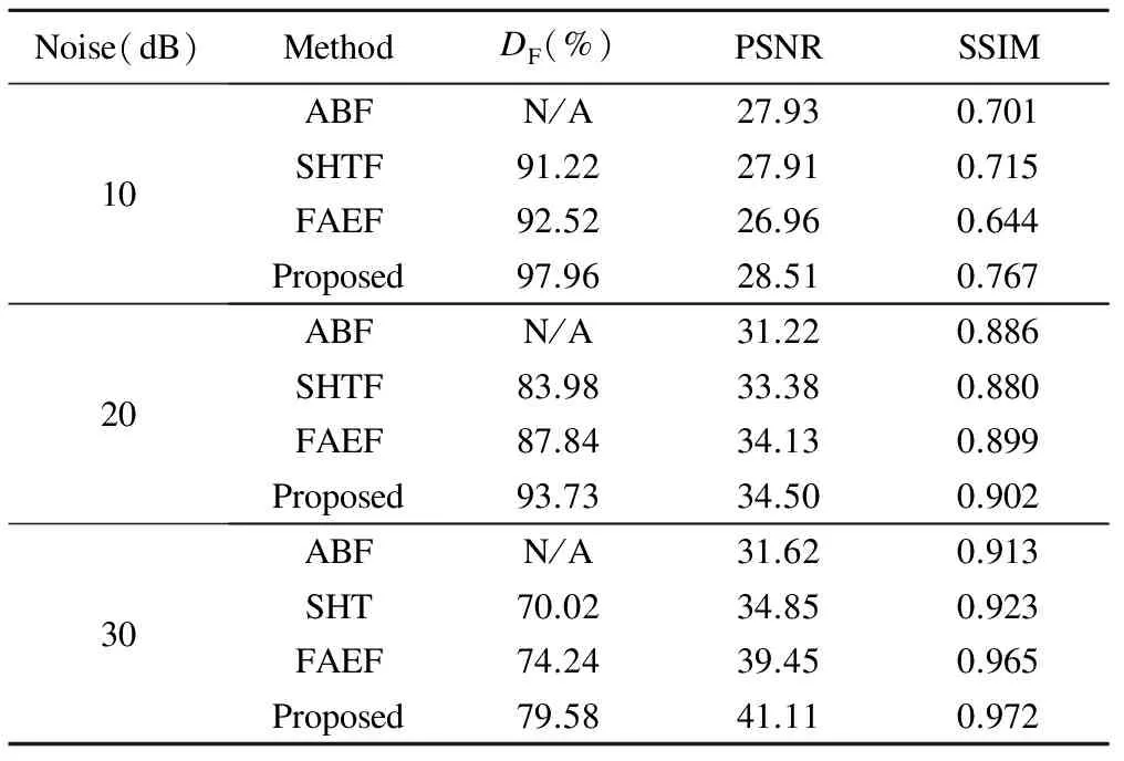
Table 2 Performance comparison with “Cameraman” image
It can be seen that the proposed algorithm can more effectively detect the noise components than the others. In particular, the noise detection accuracy of the proposed algorithm is higher and the PSNR gain of the proposed algorithm is lower when the amount of additive noise is higher. This means noise detection plays a relatively important role in the denoising problem when the amount of the noise is smaller, and that the effectiveness of the noise removal filter is important when the amount of the noise is higher. However, prior knowledge about the noise is restricted, and therefore, the estimation of noise information should be carefully taken into account. It is observed that the competitive performance of the proposed algorithm comes from the condition in which the noise detection is effectively defined by the parameters of the estimated noise, and that the adaptive filter with variable window size controls the filter strength well, so that it is possible to effectively suppress the noise without over-smoothness. In addition, it is observed that the SSIM of the SHTF is better than that of the ABF, even though the latter outperforms the former, in terms of PSNR for 10 dB noises. It is verified that these results come from the over-blurring of detailed information, using ABF.


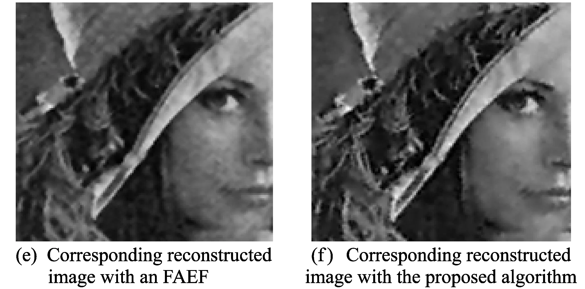
Fig.3 Experimental results with “Lena” image
Fig.3 shows the enlarged original “Lena” image, the degraded image with 10 dB Gaussian noise, the reconstructed image with ABF and the reconstructed image with the proposed algorithm. It is clear that the comparative approaches lead to over-blurring or less noise suppression. Furthermore the proposed algorithm removes the noise relatively well while preserving the detailed information and its competitiveness is clearly shown in images having higher-activity regions. Subjectively, it outperforms the other methods, which is consistently verified by Figs.4 and 5. In all cases, ABFs and SHTFs lead to overly smooth reconstructed images. On the other hand, FAEFs suppress the noise in low-activity regions relatively well, but still result in over-blurring around the high-activity regions. In general, the degree of over-smoothness of the comparative approaches increases as an image includes more high-activity regions and the amount of the noise gets smaller, since the other approaches do not carefully consider the degree of activity or the amount of noise in the detection and filtering processes.
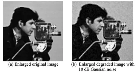

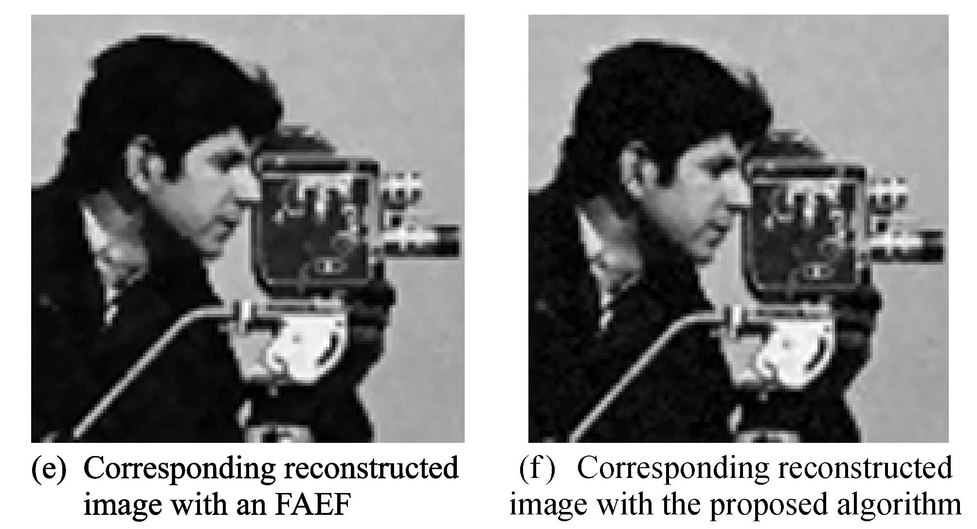
Fig.4 Experimental results with “Cameraman” image
The novelty of the proposed algorithm is that it is capable of effectively detecting the noise to adaptively suppressing it without prior information about the original image or noise, by incorporating the local statistics.
4 Conclusion
In this paper, we present an adaptive noise detection and removal algorithm. Under the assumption that an image and the additive noise have a Gaussian distribution, the statistical parameters are estimated from local information from the observed image, and the parameters are used to define the proposed noise detection function. In addition, we address the issue of an adaptive noise removal algorithm, where the filter strength is controlled by the local statistics of the estimated original image and variable filter window. The experimental results demonstrate that the proposed algorithm has the capability of reducing noise detection errors and obtaining better subjective and objective quality than do comparative approaches. Currently, we are investigating an adaptive denoising method for colour images and video sequences by incorporating a Markov random field (MRF) of the estimated noise. With such an approach, it is expected that better performance can be achieved.
[1] Gonzalez R C, Wood R E. Digital image processing. Prentice Hall Inc., Upper Saddle River, NJ, USA, 2002.
[2] Mitra S, Sicuranza G. Nonlinear image processing. Academic Press, USA, 2001.
[3] Arce G R. Nonlinear signal processing a statistical approach. John Wiley & Sons, New York, USA, 2004.
[4] Nodes T A, Gallagher N C. Mean filters: some modifications and their properties. IEEE Transactions on Acoustics Speech and Signal Processing, 1982, 30(5): 737-746.
[5] Brownrigg D. The weighted median filter. Communication of ACM, 1984, 27(8): 807-818.
[6] Ko S J, and Lee S J. Center weighted median filters and their applications to image enhancement. IEEE Transactions on Circuits and Systems, 1991, 15(4): 984-993.
[7] Zhang B, Allebach J P. Adaptive bilateral filter for sharpness enhancement and noise removal. IEEE Transactions on Image Processing, 2008, 17(5): 664-678.
[8] ZHANG Xu-ming, XIONG You-lun. Impulse noise removal using directional difference based noise detector and adaptive weighted mean filter. IEEE Signal Processing Letters, 2009, 16(4): 295-298.
[9] Lee J H, Kim Y H, Nam J H. Adaptive noise reduction algorithm based on statistical hypotheses tests. IEEE Transactions on Consumer Electronics, 2008, 54(3): 1406-1414.
[10] Nguyen T A, Hong M C. Gaussian noise image restoration using local statistics. In: Proceedings of IEEE International Conference on Consumer Electronics, Las Vegas, Nevada, USA, 2013: 153-154.
[11] Vijaykumar V R, Vanathi P T, Kanagasabapathy P. Fast and efficient algorithm to remove Gaussian noise in digital images. IAENG International Journal of Computer Science, 2010, 37(1): 300-302.
[12] Olsen S I. Noise variance estimation in images. Computer Vision, Graphics and Image Processing, 2005, 55(4): 319-323.
[13] Shin D H, Park R H, Yang S J. Block-based noise estimation using adaptive Gaussian filtering. IEEE Transactions on Consumer Electronics, 2005, 51(1): 218-226.
[14] Anderson G L, Netravali A N. Image restoration based on a subjective criterion. IEEE Transactions on System, Man and Cybernetis, 1976, SMC-6(12): 845-853.
[15] WANG Zhou, Bovik A C, Sheikh H R, et al. Image quality assessment: from error visibility to structural similarity. IEEE Transactions on Image Processing, 2004, 13(4): 600-612.
date: 2013-03-25
National Research Foundation of Korea (No. 2012M3C4A7032182)
Tuananh Nguyen (anhnt@ssu.ac.kr)
CLD number: TN911.73 Document code: A
1674-8042(2013)03-0256-07
10.3969/j.issn.1674-8042.2013.03.012
 Journal of Measurement Science and Instrumentation2013年3期
- Journal of Measurement Science and Instrumentation的其它文章
- Test on oxygen and benzene contents in gasoline by mid-infrared spectroscopy*
- Particle-filter-based walking prediction model for occlusion situations*
- Application of signal sparse decomposition in dynamic test*
- Kravchenko probability weight functions in problems of radar signals correlation processing*
- AC current automatic calibration using two different TCC designs*
- Smart decontamination device for small-size radioactive scrap metal: using abrasion pin in rotating magnetic field and ultrasonic wave cleaner*
