A discontinuum-based model to simulate compressive and tensile failure in sedimentary rock

T. Kazerani

Civil Engineering School, Faculty of Engineering, University of Nottingham, University Park, Nottingham, NG9 2NN, UK

1. Introduction

The discrete element method (DEM) has been vastly used to capture the sequences of separation and reattachment observed in the fragmentation process of brittle materials. Formulation and development of the DEM have progressed over years since the pioneering study of Cundall (1971). Jing and Stephansson (2007) have comprehensively provided the fundamentals of the DEM and its application in rock mechanics.

According to the solution algorithm used, the DEM implementations can be divided into two groups of explicit and implicit formulations. The most popular representations of the explicit DEM are the computer codes of particle flow code (PFC) and universal distinct element code (UDEC) (Itasca Consulting Group Inc,

2008a,b).

Cundall and Strack (1979) showed how the DEM could be employed to simulate behaviour of granular media, and Potyondy and Cundall (2004) showed how a similar approach could be used to model rock material as a dense packing of particles interacting at their contact points. The significant advantage of this approach is to model crack as a real discontinuity. In addition, complicated empirical constitutive behaviour can be replaced with simple particle/contact logic. In this context, stress-displacement relation of contact, i.e. micromechanical constitutive law characterizes macroscopic behaviour of the model.

Generally speaking, two types of particle geometries have been adopted to reproduce rock texture, i.e. rounded grains, vastly examined by PFC (e.g. Potyondy and Cundall, 2004; Lobo-Guerrero et al.,2006; Yoon, 2007; Schöpfer et al., 2009; Wang and Tonon, 2009;Lobo-Guerrero and Vallejo, 2010), and polygonal particles usually produced through the Voronoi diagram generator or the Delaunay triangulation algorithm (e.g. Kazerani and Zhao, 2010; Lan et al.,2010; Mahabadi et al., 2010; Kazerani et al., 2012).

Geometrically, it may be sound that the polygonal configuration may be the most representative of the mineral structure observed in crystalline rock. However, the vast majority of micromechanical models have been carried out by rounded (disc-shaped) particles.As discussed by Potyondy and Cundall (2004), modelling by using rounded particles fails in accurate reproduction of rock mechanical behaviour. They showed that calibrating PFC to the uniaxial strength gave a very low triaxial strength. In addition, predicted Brazilian tensile strength of rock was approximately 0.25 times the uniaxial compressive strength. Comparing various types of rocks,this value is unacceptably high as the ratio of tensile to compressive strength is typically reported around 0.05 to 0.1 (Hoek and Brown,1998). It is generally argued that these shortcomings are due to that the rounded particles cannot represent the irregular-shaped and interlocked grains of rock appropriately. To resolve this problem,different solutions have been proposed, e.g. flat joint formulation(two contact points per bond) in PFC provided by Itasca (Itasca Consulting Group Inc, 2008a), controlled bond density configuration in YADE (Kozicki and Donzé, 2008), and in earlier time the so-called cluster (Potyondy and Cundall, 2004) and clump logics (Cho et al., 2007). The clumped and cluster models are more convincing in reproducing the random geometry of igneous rock grains, however, inter-grain contact is still puncticular (no physical contact area). In addition, some PFC microparameters, e.g. coefficient of friction, contact modulus and parallel bond modulus, show no effect on the model response, and thus are deprived of physical sense. As Kazerani and Zhao (2010), Mahabadi et al. (2010) and Lan et al. (2010) mentioned, using polygonal particles enhances the simulation as they can represent mineral interaction efficiently.

This research aims to create a numerical model to study tensile and compressive failures in sedimentary rocks. The model involves a two-dimensional (2D) microstructural simulation based on the DEM coupled with the fracture process zone (FPZ) theory. The UDEC has been employed to implement the model. The software has been developed by creating DLLs and attaching them into the code.In addition, a pre-processor programme has been built to generate arbitrarily-sized particles based on the Delaunay triangulation algorithm (Du, 1996).

In the literature, there are two alternatives for modelling materials microstructure, i.e. (a) rigid particles with local springs(decoupled method) and (b) deformable particles in contact with zero-thickness interfaces having arbitrarily high contact stiffness(coupled method). Both the ways are of advantages and disadvantages. While in the former rigid particles causes undesired distortion in the wave travelling through the model, the latter suffers from an acute shortage of a physical definition for the interfacial stiffness. The novelty of this research is actually to open a middle way to benefit from the advantages of both the ways while avoiding the shortcomings. In this study, material microstructure has been reproduced by using elastic particles and contacts for the stiffness of which a physical definition has been provided. This definition has been developed by introducing the FPZ theory into the modelling. This is discussed in Section 2.1.1 and Appendix in detail.

2. UDEC numerical modelling

As a finite difference-discrete element coupled code, UDEC permits 2D plane-strain and plane-stress analyses. As mentioned, rock microstructure is to be modelled as an assemblage of distinct deformable particles whose boundary behaviour is dominated by the so-called contact law. In this simulation, particles are assumed to be of the same elastic properties with the rock, and the interfaces between the particles account for potential fracture. The particle assemblage is generated randomly to capture rock heterogeneity and diverse fracture patterns where each particle is individually discretized by constant strain triangular (CST) elements as presented in Fig. 1.

A perturbation within this particle assemblage, caused by an applied excitation, propagates through the whole system and leads to the particles movement. The solution scheme is identical to that used by the explicit finite difference method for continuum analysis. Solving procedure in UDEC alternates between the applications of a stress-displacement law at all the contacts, and the Newton’s second law for all the particles. The contact stress displacement law is used to find the contact stresses from the known displacements. The Newton’s second law gives the particles motion resulting from the known forces acting on them. The motion is calculated at the grid points of the CST elements within each elastic particle. Then, application of the material constitutive relations gives new stresses within the elements. Fig. 1 schematically presents the calculation cycle in UDEC together with a brief review of basic equations.

In this study, an orthotropic cohesive law has been developed for contact to capture strength, brittleness and anisotropy of rock.Orthotropy has been provided by assuming contact to have different tensile and shear behaviours in terms of strength, stiffness and ultimate displacement.

The FPZ theory has been also introduced into modelling by assuming contacts to follow a decaying stiffness at pre-failure in order to represent the damage behaviour of the FPZ. At post-failure,contact endures different stress softening depending on whether it undergoes tension or shear.

The stress σ applied on the contact surface is defined as where δeffis the contact effective displacement; ktand ksdenote the contact initial stiffness coefficients in tension and shear, respectively; and the parameters tc, cc, and φccharacterize the strength of contact which represent strength parameters of rock microstructure. They are respectively referred to as contact tensile strength,contact cohesion, and contact friction angle. δeffis defined as

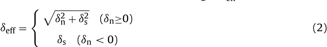
where δnand δsare the normal separation and shear sliding over the contact surface, respectively. δnis assumed positive where contact undergoes opening (tension). As Eq. (2) implies, by assumption when two bonded grains are being detached the total elongation that the bond endures is taken into account to calculate the total stress acting upon the grains boundary. This stress then is decomposed to produce normal and shear components. On the other hand,if the grains slide past each other under compression, normal and shear components of the boundary stress are calculated separately.Each of the stress components is controlled only by the corresponding contact displacement component, i.e. shear stress by δsand normal compressive stress by δn. δnis then the amount of numerical overlapping at the grains touch point (see Eq. (13)).

2.1. Definition of contact stiffness coefficient

The majority of the microstructure models by DEM or lattice simulation assume rigid particle and zero-mass local springs(decoupled mass-stiffness method). Although offering mathematical relations for the spring stiffness (e.g. Zhao et al., 2011), these models are suffering from travelling wave distortion. Alternatively there have been attempts to model material as a structure involving deformable particles in contact with zero-thickness interfaces(i.e. couples mass-stiffness method), where particles have the same elastic properties with the physical material and contact stiffness must be set in finite to avoid reduction in the global stiffness of the system. However, the implementation of this ideal assumption is practically impossible as it makes the numerical solving procedure involved with instabilities known as ill-conditioning (e.g. Babuska and Suri, 1992; Chilton and Suri, 1997). In practice, contact (interface) stiffness is arbitrarily reduced but not so much as the system global stiffness is altered noticeably (e.g. Zhai et al., 2004; Pinho et al., 2006; Elmarakbi et al., 2009). This study provides a physicalexplanation for the contact stiffness using which contact stiffness can be defined.

The FPZ theory suggests that fracture should not be regarded only as a material detachment, but the role of complex damage mechanisms at the crack-tip area must be also taken into account.Since the model does not assume damage in particle, contact must represent material deterioration within the FPZ. Thus, prior to fracture initiation, the contact (initial) stiffness coefficient is considered as

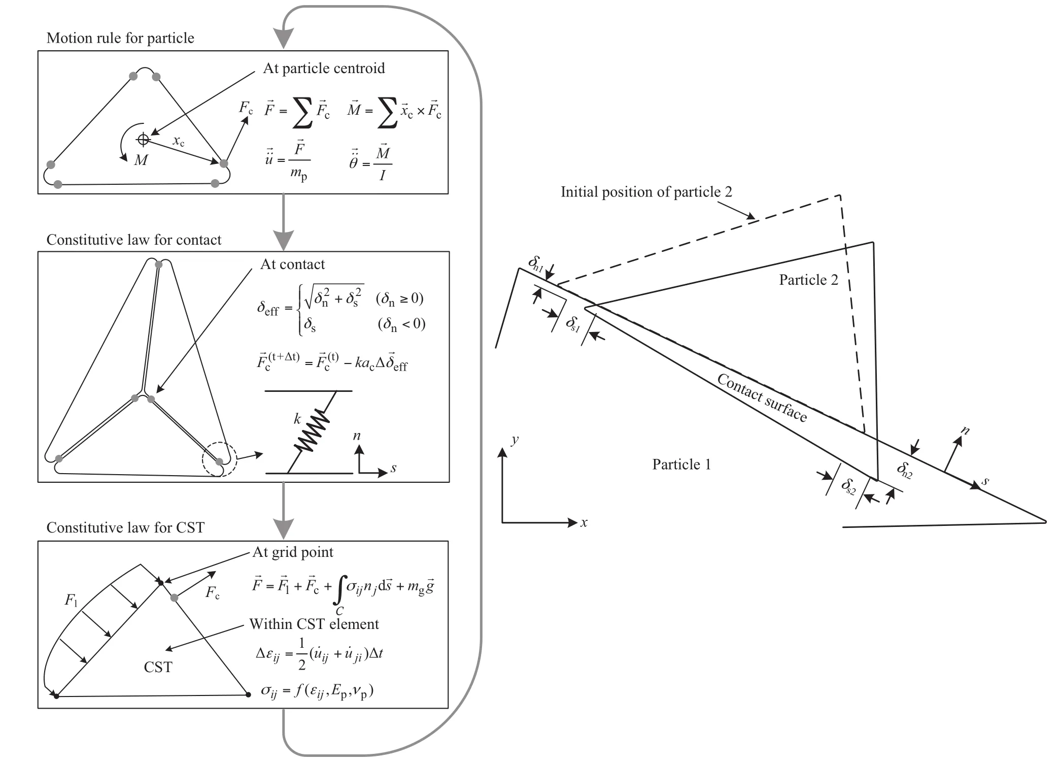
Fig. 1. Calculation cycle in UDEC (left) and representation of particle and contact used to form rock microstructure (right).

where E and G are the Young’s modulus and shear modulus of the intact material, respectively; and w is the thickness of the process zone ahead the fracture. Contact is assumed to lose stiffness gradually upon opening to represent local material deterioration as fracture initiates. Hence, a nonlinear relation is adopted to describe the contact pre-peak stress-displacement behaviour. The slope of the relation should gradually decay from the initial value at the origin as suggested by Eq. (3) to zero at the peak strength (see Fig. 2).

Two closed-form expressions are provided in Appendix for the FPZ thickness. Using them, the contact initial stiffness coefficients in plane-stress are expressed as

And in plane-strain condition, they are

where ν is the Poisson’s ratio.

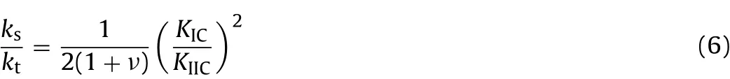
The ratio of the initial stiffness coefficients is

2.2. Stress-displacement relation of contact

The stress-displacement relation for a contact undergoing separation is expressed through

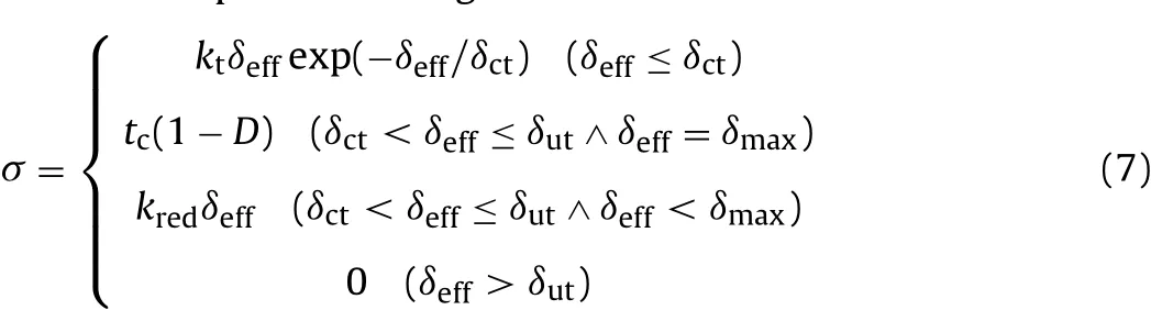
where δctis the critical tensile displacement of contact beyond which cohesive softening happens, and δutis the ultimate tensile displacement of contact at which contact loses its entire strength.As illustrated in Fig. 2a, at the peak point, we have σ = tcand δeff= δct.Substituting these values in Eq. (7) and solving it for δctyield

where e is the base of the natural logarithm.

When δeff≤ δct, stress-displacement behaviour is assumed nonlinear but elastic, i.e. the unloading and reloading paths are the same and no energy dissipates through contact opening; the governing nonlinear equation is the exponential traction-separation law described by Xu and Needleman (1996). As δeffexceeds δct,contact failure happens and it is permitted to release energy in unloading-reloading cycles. The damage variable is then defined by

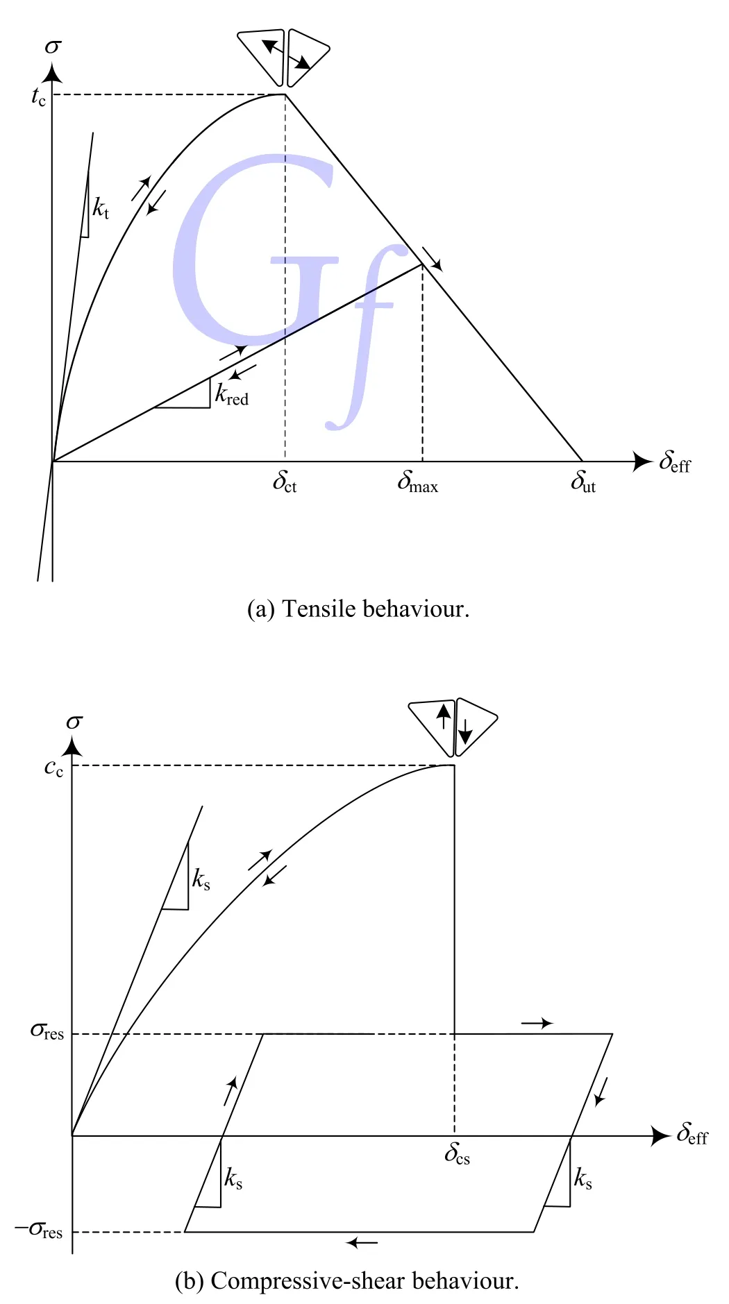
Fig. 2. Stress-displacement behaviour of a cohesive contact (arrows denote loading,unloading and reloading paths).

where δmaxis the maximum effective displacement that contact has undergone (see Fig. 2a). Fracture healing is therefore avoided as D either increases or remains constant. When δeff＜ δmax(unloading reloading cycles), contact follows a linear stress-displacement path where kredis the ratio of stress to effective displacement at δmax(see Fig. 2a).

Table 1Material properties and model microparameters.

When contact is sheared under compression, the stress dis placement law is described as where σresis the post-failure residual strength of contact which is supplied by the particle boundary friction. In shearing, no post failure softening is considered as it is assumed that the frictional effects appear instantly after contact failure.

Like tension, the critical displacement of contact in shear is calculated by

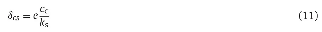
In the post-peak region, contact follows a linear unloading reloading behaviour (Fig. 2b) where the stress increment at each deformation step is calculated by

Ultimately, the normal and shear components of contact force are obtained through

where acis the contact surface area.

2.3. Contact fracture energy

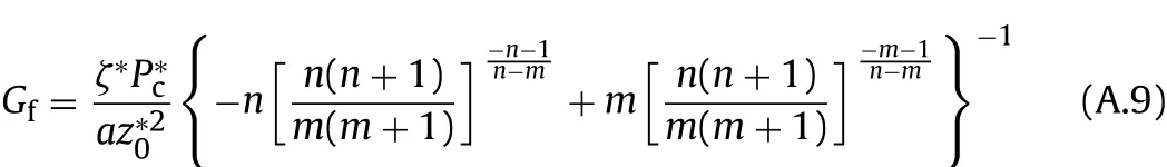
The area under the curve in Fig. 2a represents the energy needed to fully open the unit area of contact surface. Since contact is the numerical representation of fracture, this area should be equal to the fracture energy, Gf. Thus,

3. Model calibration

Table 1 lists modelling parameters which are referred to as microparameters beside the analogous material properties. A micromechanical investigation by the model requires proper selection of the microparameter by means of a calibration process in which responses of the model are compared directly to the observed responses of the physical material. These comparisons are made at the laboratory scale and include tensile and compressive tests results.

In this study, a group of simulations are generated and calibrated to Transjurane sandstone (TS). They comprise modelling samples of the Brazilian tension, uniaxial compression and triaxial compression tests. TS is the main rock type near the Jura Mountains in the Canton of Jura, Switzerland, which has been vastly tested in the rock mechanics laboratory of the Swiss Federal Institute of Technology(EPFL). Its average standard mechanical properties and mean grain size are listed in Table 2.

According to the specimens’ geometry and loading condition,a plane-strain (axisymmetric) and a plane-stress analysis are adopted for the compressive and Brazilian models, respectively.Samples are placed between two steel platens whose interfacial friction angle is assumed 5°. The contact initial stiffness coefficients obtained through Eqs. (4) and (5) are listed in Table 3.

The samples are built by particles with a mean edge size equal to the TS grains average size, i.e. 2 mm. The coefficient of variation in particle generation process is taken 0.1 mm which ends up assemblages containing particles whose dimension is between 1.4 mm and 2.6 mm. The generated compressive and tensile samples are 30 mm × 70 mm and 70 mm × 70 mm, respectively, and include 740 and 1134 particles. Fig. 3 presents two representative compressive and tensile samples.

An axial-strain increment is applied to the upper and lower platens of the systems by setting a very low axial displacement rate,i.e. 10-4m/s for a number of steps, e.g. 5000 steps. The compression is then stopped by setting the displacement rate to zero, and the systems are cycled until quasi-static equilibrium is reached.During this process, the reaction force at both the upper and lower supports is continuously recorded to generate stress-strain

curves.

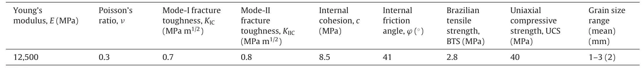
Table 2Mechanical properties of TS.

Table 3Contact initial stiffness coefficients for simulation of TS samples.

The model tensile strength is measured through the following equation:

where Fmaxis the maximum axial force recorded, D and t denote the sample diameter and thickness where t is unit for 2D simulation.

In the following, the tensile and the uniaxial compressive strengths obtained from the modelling are denoted by σtand σc,respectively, versus the laboratory measurements for the BTS and UCS of TS.

Fig. 3. Compressive and tensile samples generated by the model.

3.1. Parametric study

A parametric study is carried out to determine which microparameter has the largest impacts on which model macroscopic response. Values of ccand φcare initially given the UCS and the internal friction angle of TS, respectively, while tcis changing.Considering Eq. (A.13), the mixed-mode fracture energy, Gf, of TS is calculated as 81.5 J/m2and 87.1 J/m2for plane-strain and plane-stress, respectively. δutis then calculated by Eq. (15) for each assumed value of tcas listed in Table 4.

As expected, the model global strength is dependent of tc. Fig. 4a indicates a linear relation between tcand σt, while the uniaxial compressive strength, σc, is not sensibly changing. Note that the axes are normalized to BTS = 2.8 MPa, and UCS = 40 MPa.

By establishing a linear regression fit to the data, tcis estimated 10.97 MPa to have σt= BTS. Repetition of the simulation using this value results in σt= 2.9 MPa which is very near the TS BTS.

Given obtained tc, the sensitivity of the model to ccand φcis examined as presented in Figs. 4b and c. As seen σcis highly influenced by ccand φc, but it does not change with φcwhen φc＜ φ. On the other hand, σtis independent of ccand φc. This implies that the model global tensile strength is controlled only by the contact tensile strength and the obtained tc(= 10.97 MPa) is thus the target value.

3.2. Design of experiment

The calibration process is carried out by using a group of statistical techniques known as the design of experiment (DOE). The DOE is an efficient, structured and organized discipline to quantitatively evaluate the relations between the measured responses of an experiment and the given input variables called factors(NIST/SEMATE, 2003). The objective of the DOE is to observe how and to what extent changes in the factors influence the response variables. There are many different DOE methods. The best choice depends on the number of factors involved and the accuracy level required. Kennedy and Krouse (1999) presented the details for different DOE methods and categorized them based on the experimental objectives they meet.

The DOE begins with the definition of the experiment objectives and the selection of the input/output variables. In our purpose, the unknown microparameter (i.e. ccand φc) are chosen as the factors;and the assemblage macroscopic responses in terms of internal cohesion (c) and internal friction angle (φ) are considered as the

responses.

3.2.1. Estimation of factors range

To carry out the DOE we need to estimate the range of the factors. As Fig. 4b suggests, the contact cohesion should be about 0.5 UCS, the model demonstrates a uniaxial compressive strength close to that of TS. Hence, target ccis guessed to be between 0.25 UCS and 0.75 UCS, i.e. 10 MPa to 30 MPa. On the other hand,as the model response does not vary for φc＜ 0.5φ, 0.85φ and 1.15φ(34.85°and 47.15°) are taken the lower and upper bounds for φc.

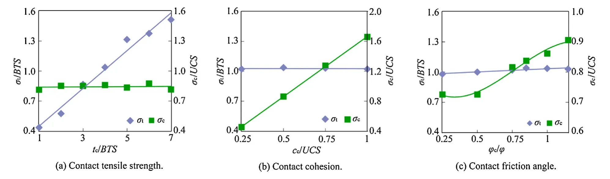
Fig. 4. Effect of contact microparameters on tensile and compressive strength of model; axes are normalized.

3.2.2. Central composite design

Depending on the level of accuracy required, a complete description of the response behaviour might need a linear, a quadratic or even a higher-order DOE. Under some circumstances,a design involving only main effects and interactions may be appropriate to describe a response surface when analysis of the results reveals no evidence of pure quadratic curvatures in the response of interest. As Fig. 4 implies, there is, however, a probability of existing interaction between the factors. Hence, a quadratic model is necessary to satisfy our objective. As an efficient quadratic model,the central composite design (CCD) is applied for the estimation of nonlinear relations between the microparameter and the model macroscopic responses.

CCD provides high quality prediction of a response surface over the entire design space, including linear, quadratic, and interaction effects. It contains an imbedded factorial or fractional factorial design with centre points that are augmented with a group of star points that allow estimation of curvature (see Table 5). If the distance from the design space centre to a factorial point is assumed±1, the distance from the design space centre to a star point will be ±α. The precise value of α depends on the number of factors involved. Since there are two factors in the model (i.e. ccand φc),α = 21/2≈ 1.414, and the number of factorial runs will be four(NIST/SEMATE, 2003).

The levels ±1 represent the upper and lower bounds of the factors. The value of each factor at the centre point is defined as the arithmetic mean of the upper and lower bound values. Given the lower and upper bounds, the centre, factorial, and star points are calculated as listed in Table 6.

CCD offers a limited number of combinations for the factors.These combinations are collected in a matrix called design matrix as listed in Table 5. This matrix is converted to the matrix of the real factors, i.e. microparameter by the transformation formula expressed at the last column in Table 6. The uniaxial and triaxial compression tests are then simulated using each set of the CCD-suggested microparameter, and the predictions for confining pressures of 0, 3 and 6 MPa are recorded in Table 7. Using the outputs of each run, internal cohesion and internal friction angle of the model are calculated as the DOE responses.

For each run, the particle assemblage is separately created. In addition, the simulations are repeated for five times with the same microparameter at the centre points (see runs 9 to 13 in Table 7).It is because the particle assemblage is generated arbitrarily andtwo numerical runs might produce slightly different results. Hence,the CCD predictively carries out this repetition to minimize the variability in modelling.

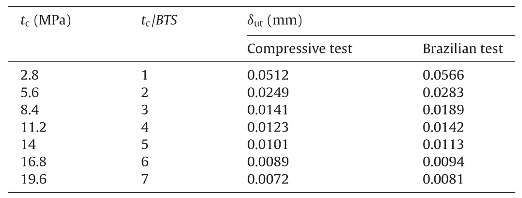
Table 4Values of contact tensile strength and corresponding ultimate displacements for TS simulation.

The targeted response parameters are statistically analyzed by applying the above data in the statistical software of JMP (Sall et al.,2007). The data are evaluated using the Fischer test, and quadratic models are generated for each response parameter using multiple linear regression analysis, analysis of variance and a backward elimination procedure. A numerical optimization procedure using desirability approach is ultimately used to locate the optimal settings of the formulation variables in view to obtain the desired response (Park and Park, 2010).

Using the data presented in Table 7, the following equations between the model macroscopic response and the coded factors are constructed eventually:

Table 5Complete design matrix for central composite design.

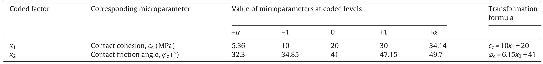
Table 6Definition of factors and numerical value of microparameter at each coded level.

Comparison of the multipliers in the above equations justifies the necessity of CCD as a quadratic model. Solving the equations for c = 8.5 MPa and φ = 41°of TS gives x1= 0.292 and x2= 0.323. These are coded factors that should be transformed to uncoded values by using the transformation equations. Eventually, cc= 22.92 MPa and φc= 42.99°are obtained as the targeted microparameters.

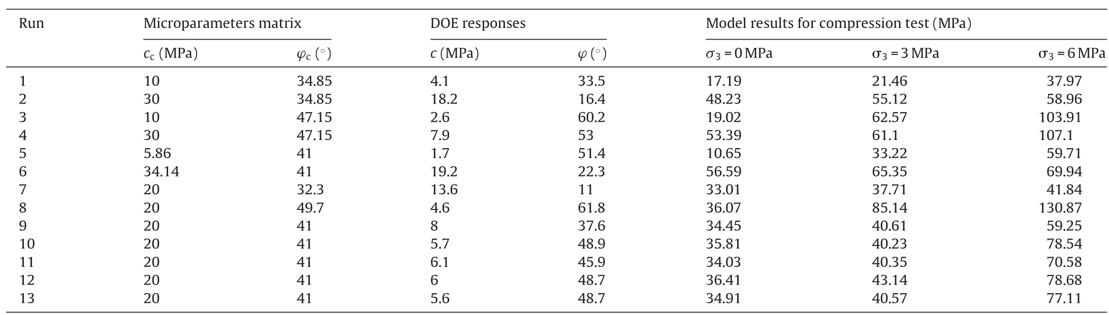
Table 7CCD-suggested design matrix and obtained results.

4. Solution verification

4.1. Quantitative comparison

The obtained microparameters are used as input for new simulations which are expected to give the closest match with the laboratory test in terms of the Young’s modulus, Poisson’s ratio,Brazilian tensile strength, uniaxial compressive strength, internal cohesion, and internal frictions angle.

Since different assemblage arrangements result in different model strengths, five models with different particle arrangements are created. Table 8 lists the results of mean, standard deviation and relative error percentage that show fair agreement with the experimental measurements where the relative error is always less than 5%.

Though the targeted microparameters are expected to provide a close match, little variations in the numerical results are unavoidable because of the inherent randomness of particle placement in the model generation. Note that this is not regarded as a disadvantage as two separate experimental tests on rock material necessarily do not lead to identical results due to rock heterogeneity. In fact, the randomness of the particle arrangement comparably represents rock heterogeneity when material anisotropy is introduced into calculation by the adopted orthotropic contact law.

Comparisons between the stress-strain curves for the laboratory test and a representative TS simulation are presented in Fig. 5a.Note that some special aspects for rock behaviour such as closure of initial flaws and pores are not captured in the modelling.This causes the stress-strain curves obtained in the simulation to be slightly different from those of the laboratory tests particularly where the initial nonlinearity is not reflected in the modelling.

The elastic constants for the laboratory testing were obtained from the middle portions of the curves where relatively linear relation between stress and strain is maintained. For numerical simulations, those are computed using stress and strain increments occurring between the start of the test and the point at which one half of the peak stress is obtained (tangent method).

Fig. 5b also plots the model predictions for the compressive and tensile strengths versus the laboratory measurements. As seen, the numerical results follow nearly the same pattern with the laboratory data. The Hoek-Brown failure envelopes are also drawn for both the numerical and experimental data where fair agreement is observed.

Table 8Experimental properties of TS versus model predictions.

4.2. Qualitative comparison

Some specific features of the simulation, e.g. failure mode and fracturing pattern, cannot be quantified efficiently. A qualitative comparison is therefore required to complete the modelling validation where the solution correctness is examined through comparing those features from laboratory results to simulation outputs.

As Wawersik and Fairhurst (1970) described, rock failure in unconfined circumstances occurs in two distinct modes of axial splitting (cleavage failure) and shear rupture (faulting). Shear faulting generally precedes axial cleavage for sedimentary soft rocks and characterizes failure initiation. Fig. 6a shows that the modelling is able to capture these phenomena where the predicted failure mode shows the typical shear faulting observed in the TS laboratory tests.

The post-failure picture for the TS Brazilian sample is plotted in

Fig. 6b. In the modelling, tensile failure starts at about the centre of the sample, then the induced fracture propagates towards loading points rapidly, and the sample is split into half ultimately. Further loading causes contacts located beneath the loading platens break.As seen, the failure features in terms of the major fault induced into the sample and the wedge-shaped zone created beneath the platen are fairly captured.

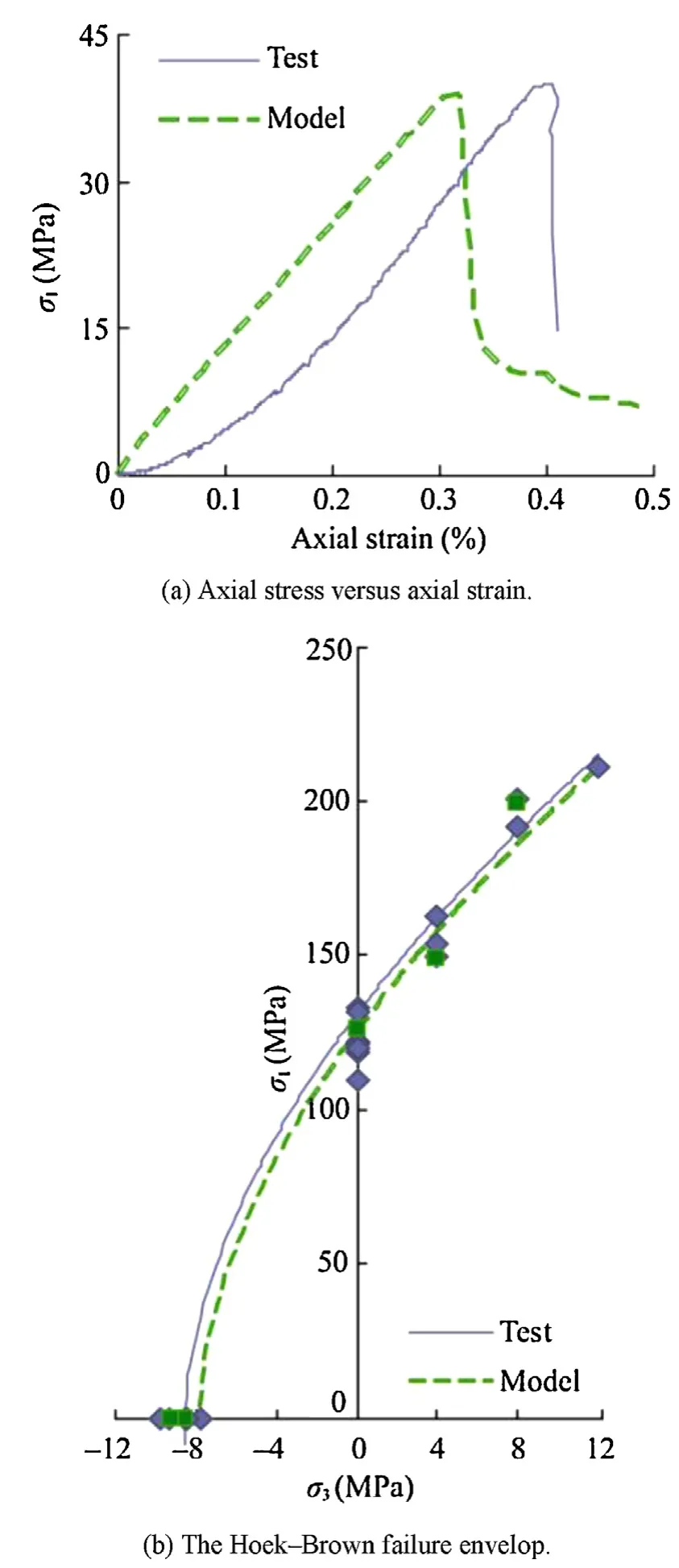
Fig. 5. Comparison of laboratory data to model predictions.

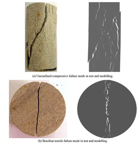
Fig. 6. Comparison of laboratory failure modes with model predictions.

5. Conclusions

A numerical model was created to represent the microstructure of sedimentary rock by considering mineral-scale geometric heterogeneity, contact orthotropy and microfailure mechanisms. The mineral-scale heterogeneity was captured by developing a Delaunay triangle generator. The discrete element programme was then used to calibrate the model such that it reproduces a variety of standard laboratory testing data. Meanwhile, statistical disciplines and mathematical developments have been employed to provide a physical understanding for the model microparameters.

The mineral-scale microparameters were shown how to control the rock macroscopic failure response. The microtensile strength was shown to have impact on peak tensile strength for the sandstone investigated where the microscale cohesion and the grain boundary friction were seen to have no significant effect. On the other hand, uniaxial and triaxial compressive strengths were observed to be controlled by the microcohesion and the grain boundary friction angle.

The presented model is a research tool to aid in understanding brittle failure processes. It was shown to provide a proper reproduction of the rocks macroscopic behaviour quantitatively and qualitatively. Besides, the study offers a straightforward and disciplined calibration procedure which is easily extendable to use in other discontinuum-based microstructural simulations. It also provides close-formed expressions for the stiffness coefficient,tensile strength and cohesion of the contact showing how the material macroscopic properties are related to the microstructural parameters.

This modelling has been implemented in 2D while the actual physical failure events proceed in a full 3D space. Therefore, the continuation of this simulation through its extension to 3D could provide us with a more clear understanding of the failure phenomenon. The presented contact model and the related DLLs have been developed in 3D, therefore, they can be used in 3DEC (the 3D version of UDEC) in future as planned by the author.

Acknowledgement

The author is grateful to Prof. Jian Zhao, the head of “le Laboratoire de Mécanique des Roches” (LMR) of EPFL, for his valuable comments. The laboratory data used have been supplied by the LMR test room too. The author also would like to thank Mr. Jean-Franc¸ ois Mathier for providing the test data. The anonymous reviewers’comments are also appreciated.

Appendix A. An estimation for thickness of fracture process zone

A material cracks when sufficient stress and energy are applied to break the inter-molecular bonds. These bonds hold the molecules together and their strength is supplied by the attractive forces between the molecules. Many equations have been proposed to formulate this force and its potential energy. The Lennard-Jones’potential (Griebel et al., 2007) is a simple and extensively used function:

Fig. A.1. Lennard-Jones’ potential for real and homogenized material (left and middle), and homogenized inter-molecular force (right).

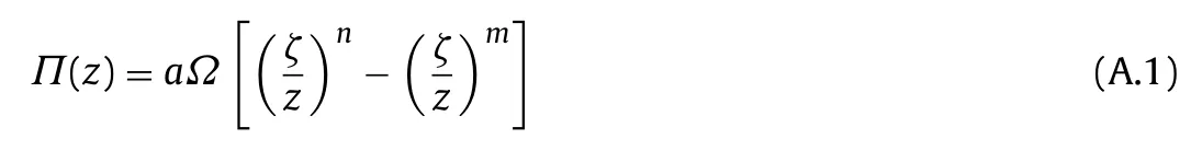
where z denotes the separation distance between two adjacent molecules, and

The depth of the potential, Ω, describes the energy needed to break the bond and thereby the strength of the molecular force(Fig. A.1). It is called bond energy. The value ζ parameterizes the zero crossing of the potential; the integers m and n depend on the material molecular nature and are more commonly among 6 to 16.

On close inspection, all real materials show a multitude of heterogeneities even if they macroscopically appear to be homogeneous. These deviations from homogeneity may exist in form of cracks, voids, particles or regions of a foreign material

, layers or fibres in a laminate, grain boundaries or irregularities in a crystal lattice. Heterogeneities of any kind can locally act as stress concentrators and thereby lead to the formation and coalescence of microcracks or voids as a source of progressive material damage. To take these microstructural defects into account, a homogenization approach is adopted by assuming the process zone as the representative volume element across which the fine-scale heterogeneous microstructure is “smeared out” and the material is described as homogeneous with spatially constant effective properties. The latter then accounts for the microstructure in an averaged sense. They,for our purpose, include the bound energy and zero crossing of the potential. As illustrated in Fig. A.1, the effective potential of the homogenized process zone is thus formulized by

where the parameters superscripted by asterisk denote the effective ones.

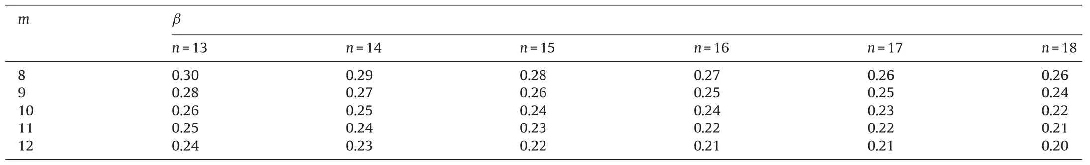
Table A.1Values of β for common values of m and n.

As the potential derivative with respect to z, the homogenized inter-molecular force P∗(z) is written as

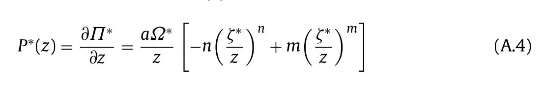
The peak value of the homogenized inter-molecular force, which is called effective cohesive force, P∗c, takes place at z∗mas shown in

Fig. A.1. Note that P∗cis significantly smaller than the actual peak molecular force in the physical material, as it includes an average effect of the entire material microdefects. Solving the derivative of P∗(z) for z:

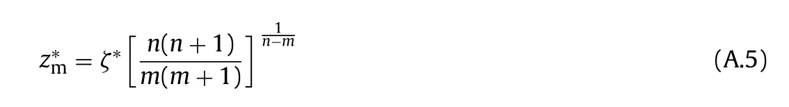
Substituting z∗minto Eq. (A.4) leads to

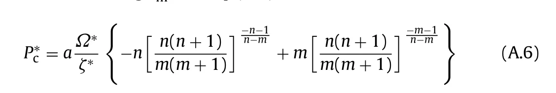
The homogenized equilibrium spacing between two molecules(z∗0) occurs when the potential energy is at a minimum or the force is zero. Solving Eq. (A.4) for z provides

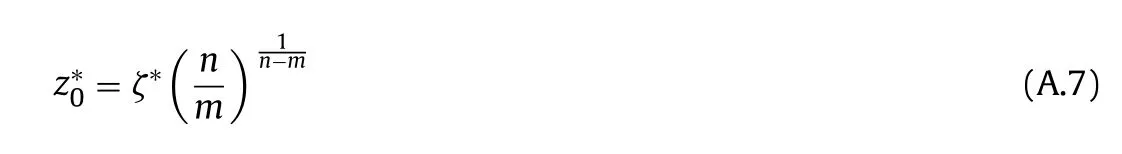
A tensile force is required to increase the separation distance from the homogenized equilibrium value. If this force exceeds the effective cohesive force, the bond is completely severed. The homogenized material then cracks and stress in a width equal to z∗0is released. This means that z∗0(which is significantly larger than real molecular equilibrium spacing) represents the homogenized process zone thickness (w), i.e. w = z∗0.

When a bond breaks, a quantity of energy equal to Ω∗is dissipated. The accumulation of these energies over the process zone surface supplies the energy dissipation through fracturing.Therefore, the Griffith’s fracture energy, Gf, defined as the rate of energy release per unit cracked area, is expressed as

Substituting Ω∗obtained from Eq. (A.6) into the above relation yields

On the other hand, the effective tensile strength of the homogenized material which represents the actual tensile strength of the material is estimated by

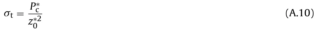
Substituting Pc∗from Eq. (A.9) and z0∗from Eq. (A.7) into Eq. (A.10)and solving it for z0∗which actually represents the homogenized fracture process zone thickness, w, yields

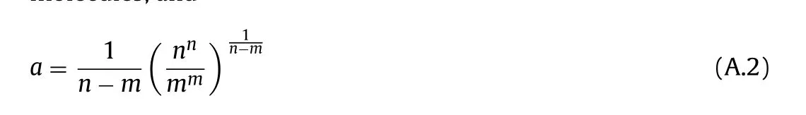
where

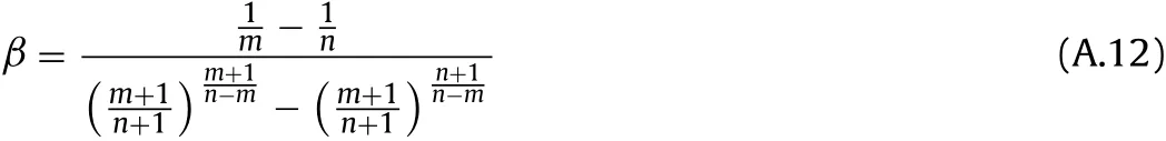
depends on the integers m and n. Table A.1 shows that β is relatively constant at 0.25 for common values of m∈(8,12) and n∈(13,18).

In mixed mode fracturing, we have

where˜E = E for plane-stress, and˜E = E/(1 - ν2) for plane-strain.Given β = 0.25, for fracturing under pure tension, we have

and under pure sliding

Babuska I, Suri M. On locking and robustness in the finite-element method. Siam Journal on Numerical Analysis 1992;29(5):1261-93.

Chilton L, Suri M. On the selection of a locking-free hp element for elasticity problems. International Journal for Numerical Methods in Engineering 1997;40(11):2045-62.

Cho N, Martin CD, Sego DC. A clumped particle model for rock. International Journal of Rock Mechanics and Mining Sciences 2007;44(7):997-1010.

Cundall PA. A computer model for simulating progressive, large scale movements in blocky rock systems. In: Proceedings of the International Symposium on Rock Fracture. International Society for Rock Mechanics (ISRM); 1971.p. 129-36.

Cundall PA, Strack O. A discrete numerical model for granular assemblies. Geotechnique 1979;29(1):47-65.

Du C. An algorithm for automatic Delaunay triangulation of arbitrary planar domains. Advances in Engineering Software 1996;27(1/2):21-6.

Elmarakbi AM, Hu N, Fukunaga H. Finite element simulation of delamination growth in composite materials using LS-DYNA. Composites Science and Technology 2009;69(14):2383-91.

Griebel M, Knapek S, Zumbusch G. Numerical simulation in molecular dynamics:numerics, algorithms, parallelization, applications. Springer; 2007.

Hoek E, Brown ET. Practical estimates of rock mass strength. International Journal of Rock Mechanics and Mining Sciences 1998;34(8):1165-86.

Itasca Consulting Group, Inc PFC user manual. Minneapolis, MN: Itasca Consulting Group, Inc., 2008.

Itasca Consulting Group, Inc UDEC user manual. Minneapolis, MN: Itasca Consulting Group, Inc., 2008.

Jing L, Stephansson O. Fundamentals of discrete element methods for rock engineering: theory and application. Elsevier; 2007.

Kazerani T, Zhao J. Micromechanical parameters in bonded particle method for modelling of brittle material failure. International Journal for Numerical and Analytical Methods in Geomechanics 2010;34(18):1877-95.

Kazerani T, Yang Z, Zhao J. A discrete element model for predicting shear strength and degradation of rock joint by using compressive and tensile test data. Rock Mechanics and Rock Engineering 2012;45(5):695-709.

Kennedy M, Krouse D. Strategies for improving fermentation medium performance: a review. Journal of Industrial Microbiology and Biotechnology 1999;23(6):456-75.

Kozicki J, Donzé FV. A new open-source software developed for numerical simulations using discrete modelling methods. Computer Methods in Applied Mechanics and Engineering 2008;197(49/50):4429-43.

Lan H, Martin CD, Hu B. Effect of heterogeneity of brittle rock on micromechanical extensile behavior during compression loading. Journal of Geophysical Research 2010;115(B1):B01202.

Lobo-Guerrero S, Vallejo LE, Vesga LF. Visualization of crushing evolution in granular materials under compression using DEM. International Journal of Geomechanics 2006;6(3):195-200.

Lobo-Guerrero S, Vallejo LE. Fibre-reinforcement of granular materials: DEM visualisation and analysis. Geomechanics and Geoengineering 2010;5(2):79-89.

Mahabadi O, Cottrell B, Grasselli G. An example of realistic modelling of rock dynamics problems: FEM/DEM simulation of dynamic Brazilian test on barre granite.Rock Mechanics and Rock Engineering 2010;43(6):707-16.

NIST/SEMATECH. 2003. E-handbook of statistical methods. http://www.itl.nist.gov/div898/handbook/

Park HJ, Park SH. Extension of central composite design for second-order response surface model building. Communications in Statistics-Theory and Methods 2010;39(7):1202-11.

Pinho ST, Iannucci L, Robinson P. Formulation and implementation of decohesion elements in an explicit finite element code. Composites Part A. Applied Science and Manufacturing 2006;37(5):778-89.

Potyondy DO, Cundall PA. A bonded-particle model for rock. International Journal of Rock Mechanics and Mining Sciences 2004;41(8):1329-64.

Sall J, Creighton L, Stephens M, Creighton L. JMP Start Statistics: A Guide to Statistics and Data Analysis Using JMP. Fourth Edition Cary, North Carolina: SAS Institute;

2007.

Schöpfer MPJ, Abe S, Childsa C, Walsha JJ. The impact of porosity and crack density on the elasticity, strength and friction of cohesive granular materials: Insights from DEM modelling. International Journal of Rock Mechanics and Mining Sciences

2009;46(2):250-61.

Wang Y, Tonon F. Modeling Lac du Bonnet granite using a discrete element model. International Journal of Rock Mechanics and Mining Sciences 2009;46(7):1124-35.

Wawersik WR, Fairhurst C. A study of brittle rock fracture in laboratory compression experiments. International Journal of Rock Mechanics and Mining Science and Geomechanics Abstracts 1970;7(5):561-4.

Xu XP, Needleman A. Numerical simulations of dynamic crack growth along an interface. International Journal of Fracture 1996;74(4):289-324.

Yoon J. Application of experimental design and optimization to PFC model calibration in uniaxial compression simulation. International Journal of Rock Mechanics and Mining Sciences 2007;44(6):871-89.

Zhai J, Tomar V, Zhou M. Micromechanical simulation of dynamic fracture using the cohesive finite element method. Journal of Engineering Materials and Technology 2004;126(2):179-91.

Zhao GF, Fang J, Zhao J. A 3D distinct lattice spring model for elasticity and dynamic failure. International Journal for Numerical and Analytical Methods in Geomechanics 2011;35(8):859-85.