On-line Modeling of Ship Maneuvering Motion based on Support Vector Machines

XU Feng,ZOU Zo-jin,b,YIN Jin-chun

(a.School of Naval Architecture,Ocean and Civil Engineering;b.State Key Laboratory of Ocean Engineering,Shanghai Jiao Tong University,Shanghai 200240,China)

1 Introduction

Mathematical modeling of ship maneuvering motion is of great significance for prediction and assessment of ship maneuverability.The time varying characteristics of ship maneuvering motion at sea require a real-time prediction of ship maneuverability,in which on-line modeling plays an important role.There are four common-used methods for ship maneuvering modeling,i.e.,captive model test,empirical estimation,theoretical or numerical calculation,and system identification(SI)based on free running model tests or full-scale trials.Along with the development of modern experiment and measurement techniques,the fourth modeling method has been increasingly applied in ship maneuvering modeling.Compared with other modeling methods,it is more suitable for on-line modeling.

The traditional SI methods include Least Square Method(LSM),Extended Kalman Filter(EKF),and so on.In recent years,artificial intelligence methods such as Artificial Neural Network(ANN)and Support Vector Machines(SVM)are widely used.Haddara,Hess and others[1-2]have successfully applied ANN for modeling of ship maneuvering.Luo and Zou et al[3-4]have made a lot of efforts on modeling of ship maneuvering by using SVM.

SVM methods include Least Square SVM(LS-SVM),ε-SVM,υ-SVM,and so on.Its algorithms contain batch algorithm and on-line algorithm.Jachims,Lin and others[5-6]have intensively studied on batch algorithm,and two simple and effective software packages for SVM calculation,LIBSVM and SVMlight,were developed.Laskov,Martion,Cauwenberghs and others[7-9]studied on-line SVM algorithm.

On-line SVM algorithm can be categorized into two types,i.e.,the incremental one and sliding window one.This paper makes an effort on on-line modeling of ship maneuvering by using incremental LS-SVM.The incremental LS-SVM is deduced from LS-SVM by means of transformation of kernel function matrix.It is then proofed by simulation test and free-running model test.Firstly,the simulation tests are carried out by using the linear hydrodynamic model,in which the hydrodynamic derivatives are obtained from full-scale trial.By analyzing the data of simulation test,the hydrodynamic derivatives are on-line identified;and the identified results are compared with the full-scale trial results.Secondly,the maneuverability indexes K and T in the first-order response model are on-line identified by analyzing the data of freerunning model tests.Then the yaw motion is predicted based on the identified response model.The predicted yaw rates are compared with those of free-running model tests.

2 Incremental LS-SVM

SVM methods include standard form and improved form.LS-SVM used in this paper is one of the improved forms.In this section,incremental LS-SVM is deduced from LS-SVM by kernel function matrix’s recursion.

2.1 Mathematical description of LS-SVM

The feature space representation of LS-SVM is given by

Optimization problem

Subject to

where C is rule factor,e is regression error.

Lagrange function is defined for objective function and constraint conditions,

where,αiis Lagrange multiplier.Partial derivative with respect to w,b,e and α gives:

Substituting the first and second formulas in Eq.(5)into the fourth,subject to the third,gives

Regression estimation function can be obtained once Eq.(6)is solved,

For the problem of motion parameter identification,linear kernel functionis commonly adopted.

2.2 Incremental LS-SVM

With regard to incremental LS-SVM,the sample number for identification increases progressively.Along with the time updating,a new sample is added to the sample set{x,y}every time.Consequently,the sample set can be described as a function of time step t,i.e.{x（t）,y（t）},where,x（t）=［x1,x2,…,xt］,y（t）=［y1,y2,…,yt］.In this way,the kernel function matrix Ω,Lagrange multiplier α and offset b are all functions of t.They can be described as follows:

Then Eq.(7)can be represented as follows:

It follows from Eq.(9):

Assuming P（t）=Γ（t）-1and multiplying Eq.(11)with eTP（t）,we obtain

Solving Eq.(13),we obtain

Substituting Eq.(10)into Eq.(12),it gives,

Substituting Eq.(14)into Eq.(11),α（t）can be determined as,

From Eq.(14)and Eq.(15),it is not difficult to find out that the essential question for online identification with incremental LS-SVM is solving P（t）.If the sample size is very big,to solve the inversion of Γ for acquiring P（t）is obviously troublesome.Therefore,a method for solving P（t）is proposed based on the matrix transformation theory in the following.

The kernel function matrix is t×t square matrix at the time step t.It gives

At the time step t+1,a new sample（xt+1,yt+1）is added to the sample set and the sample size turns into t+1.Consequently,Γ（t）turns into Γ（t+1）,which is a matrix of（t+1）×（t+1）.

Comparing Γ（t）with Γ（t+1）,Γ（t+1）can be described as follows:

where,W（t+1）=［k（x1,xt+1）,…,k（xt,xt+1）］T,w（t+1）=k（xt+1,xt+1）+1/C.

With regard to matrix A,if it can be described as partitioned matrixand both A-1andexist simultaneously,then it can be decomposed as follows[10]:

According to Eq.(18)and Eq.(19),P（t+1）is solved:

Thus the recursive algorithm for incremental LS-SVM is completed.Summarizing the above deducing process,the algorithm for incremental LS-SVM can be described as follows:

Step 1:Set the initial sample size for system identification and t must be higher than 2.

Step 2:Calculate P（t）,b（t）and α（t）,and update the time step t to t+1.

Step 3:Collect new sample（xt+1,yt+1）,and calculate P（t+1）by using Eq.(20).

Step 4:Calculate b（t+1）and α（t+1）based on Eq.(14)and Eq.(15).

Step 5:Update the time step t to t+1 and go to Step 3.

3 Validation based on simulation test

To verify the incremental LS-SVM,linear hydrodynamic mathematical model is adopted to simulate ship maneuvering motion.The mathematical model is given as:

To normalize Eq.(21),we rewrite it in the form as follows:

where,v,r,ψ and δ denote sway speed,yaw rate,heading angle and rudder angle,θi（i=1,2,…10）are normalized hydrodynamic derivatives including inertial force,viscous force and rudder force,α=π/180,V is ship speed,L is ship length.According to parameter’s identifiable theory,inertial force derivatives including θ1,θ2,θ3and θ4are assumed known.

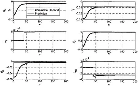
Hydrodynamic derivatives obtained from the full-scale trial of a 210 000 DWT tanker[11]are applied to simulate ship’s 5°/5°zigzag test by using fourth order Runge-Kutta method.The sample number is 200 and the sample interval is 3 s.The rule factor is set as 3.0×105and the initial sample size is 2.Then hydrodynamic derivatives are identified varying with sample size.The variable derivatives are shown in Fig.1,

Fig.1 Identified parameters with variable sample size

From Fig.1,it is easy to find that the derivatives are all very close to the expected values when the sample size exceeds 60.Tab.1 shows the identified parameters in the case when the sample size is 60.

Tab.1 Identified parameters with the sample size of 60

4 Validation based on free-running model test

In order to further verify the incremental LS-SVM in on-line identification,the KVLCC free-running model test data of Hamburg Ship Model Basin(HSVA)[12]are adopted to identify on-line the first order linear response model.This scale ratio of the ship model is 1:45.714.Its geometry and motion parameters are shown in Tab.2.

Tab.2 Main model parameters

The first order linear response model is rewritten in the form:

where,K and T are the maneuverability indexes.

Discretizing Eq.(23)gives,

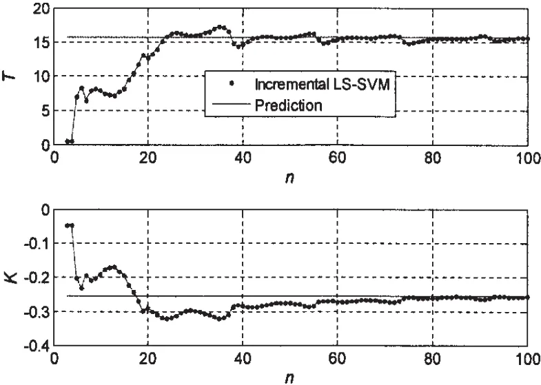
To obtain the maneuverability indexes,three sets of data including 25°/5°,15°/5°and 10°/1°zigzag tests are processed in batches at first and mean maneuverability indexes are gained.The results are K=-0.255 9 and T=15.681 6.Then 15°/5°zigzag test data are utilized to identify on-line the first order linear response model.The sample number is 100 and the sample interval is 1.5 s.Incremental LS-SVM is applied to identify the maneuverability indexes and the variation of K and T are shown in Fig.2.It is not difficult to find out that both K and T are converged to the expected value when the size of samples exceeds 50.

Fig.2 Identified maneuverability indexes with variable sample size

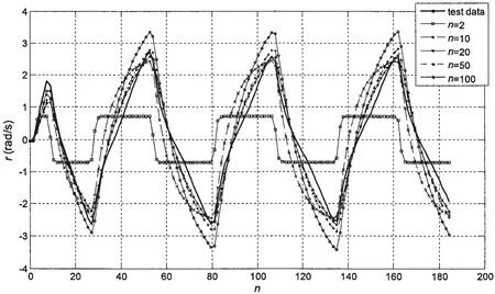
Choosing 5 couples of maneuverability indexes with n=2,10,20,50 and 100,Eq.(24)is adopted to predict the yaw rate.The results are shown in Fig.3.It is shown that the predicted results are constantly close to test data with the increase of sample size.The predicted results are distorted when the sample size is 2,but they are close to the test data when the sample size reaches 50.

Fig.3 Yaw rates with changed sampling numbers

5 Conclusions

Incremental LS-SVM is deduced and applied for on-line modeling of ship maneuvering.By simulating ship’s linear hydrodynamic model,hydrodynamic derivatives are on-line identified.The identification results are very close to test data of full scale trials,which verifies the validation of incremental LS-SVM in on-line modeling of ship maneuvering.Then incremental LS-SVM is adopted to identify the first order linear response model by using free-running model test data and yaw rates are predicted based on the identification results.The prediction results are all in good agreement with the free-running model test data,which further conforms the effectiveness of incremental LS-SVM in on-line modeling of ship maneuvering.

[1]Haddara M R,Wang Y.Parametric identification of maneuvering models for ships[J].International Shipbuilding Progress,1999,46(445):5-27.

[2]Hess D,Faller W,Lee J.Real-time nonlinear simulation of maneuvers for US navy combatant DTMB 5415[C]//SIMMAN 2008,Workshop on Verification and Validation of Ship Manoeuvring Simulation Methods.Copenhagen,Denmark,April 2008.

[3]Luo W L,Zou Z J.Parametric identification of ship maneuvering models by using support vector machines[J].Journal of Ship Research,2009,53(1):19-30.

[4]Luo W L,Zou Z J,Li T S.Application of support vector machine to ship steering[J].Journal of Shanghai Jiao Tong University(Science),2009,14(4):462-466.

[5]http://www.csie.ntu.edu.tw/～cjlin/libsvm/[EB/OL].

[6]http://www.cs.cornell.edu/People/tj/svm_light/[EB/OL].

[7]Laskov P,Gehl C,Krüger S,Müller K.Incremental support vector learning:Analysis,implementation and applications[J].Journal of Machine Learning Research,2006(7):1909-1936.

[8]Maitin M.On-line support vector machines for function approximation[R].Technical Report,Universitat Politècnica de Catalunya,2002.

[9]Cauwenberghs G,Poggio T.Incremental and decremental support vector Machine learning[J].Advances in Neural Information Processing Systems In NIPS,2000(13):409-415.

[10]Zhang J K.Linear model’s parameters estimation method and its improvement[M].Changsha:National University of Defense Technology Press,1992.(in Chinese)

[11]Åström K J,Källström C G.Identification of ship steering dynamics[J].Automatica,1976(12):9-22.

[12]http://www.simman2008.dk/[DB/OL].SIMMAN 2008,Workshop on Verification and Validation of Ship Manoeuvring Simulation Methods.Copenhagen,Denmark,April 2008.