End-to-End Paired Ambisonic-Binaural Audio Rendering

Yin Zhu , Qiuqiang Kong , Junjie Shi , Shilei Liu , Xuzhou Ye , Ju-Chiang Wang , Hongming Shan ,,, and Junping Zhang , ,

Abstract—Binaural rendering is of great interest to virtual reality and immersive media.Although humans can naturally use their two ears to perceive the spatial information contained in sounds, it is a challenging task for machines to achieve binaural rendering since the description of a sound field often requires multiple channels and even the metadata of the sound sources.In addition, the perceived sound varies from person to person even in the same sound field.Previous methods generally rely on individual-dependent head-related transferred function (HRTF)datasets and optimization algorithms that act on HRTFs.In practical applications, there are two major drawbacks to existing methods.The first is a high personalization cost, as traditional methods achieve personalized needs by measuring HRTFs.The second is insufficient accuracy because the optimization goal of traditional methods is to retain another part of information that is more important in perception at the cost of discarding a part of the information.Therefore, it is desirable to develop novel techniques to achieve personalization and accuracy at a low cost.To this end, we focus on the binaural rendering of ambisonic and propose 1) channel-shared encoder and channel-compared attention integrated into neural networks and 2) a loss function quantifying interaural level differences to deal with spatial information.To verify the proposed method, we collect and release the first paired ambisonic-binaural dataset and introduce three metrics to evaluate the content information and spatial information accuracy of the end-to-end methods.Extensive experimental results on the collected dataset demonstrate the superior performance of the proposed method and the shortcomings of previous methods.

I.INTRODUCTION

BINAURAL rendering [1] creates realistic sound effects for headphone users by precisely simulating the source location of the sounds.It has broad applications in various entertainment scenarios such as music, movies, games, as well as virtual/augmented/mixed reality, and even metaverses[2]-[9].Usually, binaural rendering involves two sequential steps: 1) utilizing a multichannel device to capture the sound field and 2) transforming this multichannel sound into a stereo sound that can be perceived by human ears.There are two indispensable functions in binaural rendering.One is headrelated transfer function (HRTF), which describes how a sound from any location is transformed by the head and ears before reaching the ear canal [1].The other is the time domain representation of HRTF, named head-related impulse response(HRIR), which is used more commonly than HRTF.Considering that HRTF and HRIR are essentially the same, for convenience, they will not be strictly distinguished unless necessary.

The existing methods for binaural rendering of ambisonics can be summarized into two categories: 1) virtual loudspeaker-based methods use the virtual loudspeaker layout and HRIRs to simulate the effect of loudspeaker playback [2]-[4]and 2) spherical harmonic-based methods use spherical harmonic functions and HRIRs to directly calculate the binaural signals [5]-[9].Figs.1(a) and 1(b) show the workflows of these two methods.Note that each of them has its respective drawbacks.The virtual loudspeaker-based methods demand considerable computation and memory resources because of the matrix multiplication and convolution operation involved,and the spherical harmonic-based methods introduce additional errors due to HRTF approximation, interpolation, or truncation [7].

In addition, these methods have two common disadvantages: 1) high personalization cost for users, and 2) low numerical accuracy, which are detailed as follows.

a)High personalization cost: Both methods require special HRTF measurements for the specific user to achieve personalized effects.However, measuring HRTF is costly.Specifically, the measurement process of HRTF has to be performed in an anechoic chamber, and the sound sources at different positions have to be measured repeatedly and separately.Taking the 3D3A HRTF dataset [10] as an example, they measured the HRTF of 648 positions for 38 subjects.

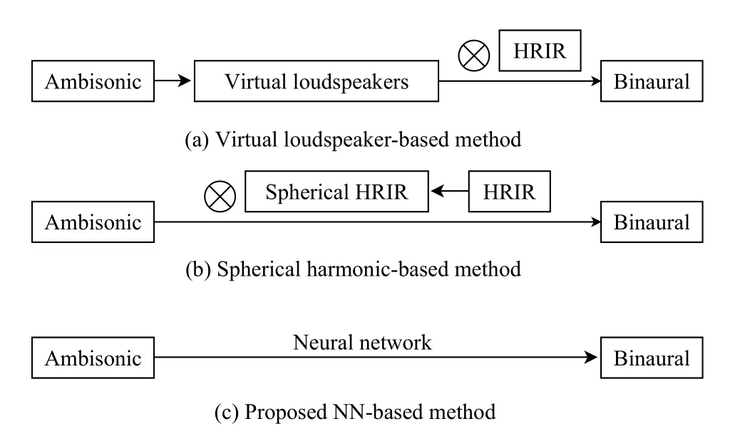
Fig.1.Workflows of traditional methods and proposed neural networkbased method (⊗ for the convolution operation).The rectangle entity represents a signal in time domain, and the bold arrow indicates that this is a core step in the algorithm.

b)Low numerical accuracy: The optimization objectives of these two types of methods are mostly heuristic and inspired by duplex theory [11].As a persuasive theory, duplex theory explains how humans can locate sounds by using two cues:Interaural time difference (ITD) and interaural level difference (ILD).However, duplex theory cannot provide a specific mathematical model of the human sound localization mechanism.Moreover, the measurement accuracy of HRTFs and the optimization method that affects the rendering results by acting on HRTFs will further amplify the loss of numerical accuracy.

In contrast, we believe that end-to-end methods can avoid these two issues because they do not require HRTF and its optimization target is directly based on the rendering result.

However, there are different problems to overcome:

1) Lack of datasets.End-to-end methods require paired ambisonic and binaural signals.The dynamic systems of the ambisonic signals generated by different sound fields will have significant differences that cannot be ignored, and the binaural signals will vary from person to person.Therefore, it is the best for the dataset to correspond to a specific scenario and individual.

2) Difficulty in learning the spatial information of ambisonic signals.Spatial information in sound is less considered in sound-related tasks because their data are a single channel or synthesized multichannel sound.However, ambisonic signals are multichannel sounds in a real sound field.

3) Difficulty in measuring the spatial information of binaural signals.End-to-end methods require a differentiable loss function to measure the similarity between the predicted binaural signal and the true binaural signal in spatial information.The mentioned ILD and ITD are not easy to calculate mathematically.Although it is obvious for single-source signals(ILD can be obtained by comparing the amplitude of the peaks, and ITD can be obtained by comparing the position of the peaks), there is currently no good calculation method for multiple-source signals, since the interference between signals from different sources can affect the amplitude and position of the peak.

To overcome these problems, we propose an end-to-end deep learning framework for the binaural rendering of ambisonic signals as follows:

1) We collect a dataset that simulates a band playing scenario for the Neumann KU100 dummy head.

2) We propose a model architecture called SCGAD (spatialcontent GRU-Attention-DNN) that divides the features of an ambisonic signal into the spatial feature and content feature.We assume that the different channels of ambisonic signals correspond to different perspectives of the sound field.For learning spatial features, we notice that ILD and ITD are essential features generated by comparing channels.Therefore, we propose a channel-shared encoder and a channelcompared attention mechanism.For learning content features,we adopt a common but effective choice: Gated recurrent unit(GRU).GRU is a category of recurrent neural networks(RNNs) that can learn the features that change over time.Since our model does not change the size of the feature when processing the feature, then, we can combine the spatial feature and content feature through a concatenation operation along the channel axis.Finally, we use a dense neural network (DNN) to process the combined feature.

3) We provide a differentiable definition of ILD of multisource binaural signals, which can be used for loss functions.This definition is based on the Fourier Transform, i.e., the sound source of binaural signals is uniformly regarded as the basis of the Fourier transform.In addition, we also provide a mathematical definition of the ITD of multi-source binaural signals, but it is non-differentiable and can only be used for evaluation.

The main contributions of this paper are summarized as follows.

1) We view the multiple channels of surround sound as different perspectives of the same sound field.Based on this, we propose to use a channel-shared encoder to learn the spatial feature of each channel separately.

2) We regard spatial feature learning as a comparison process between channels.To this end, we propose an attention mechanism that compares channels pairwise.

3) Duplex theory considers that ILD and ITD are the key to sound localization.Therefore, we propose a loss function quantifying ILD to deal with spatial information.For ITD, we did not find a quantifying method that is numerically stable and differentiable, but we considered it during evaluation.

In the remainder of this paper, we survey related works in Section II.We introduce our proposed methods in detail in Section III.A comprehensive experiment is performed in Section IV.We discuss possible questions in Section V.Finally,we conclude the paper in Section VI.

II.RELATED WORK

In this section, we will briefly review some works related to the ambisonic.

To render sound fields more efficiently in both computing and storage than other sound formats that record information pertaining to point sound sources, Gerzon [12] proposed ambisonics to capture the entirety of the sound field without regarding the signal and position of any particular point in the field.However, this characteristic prevents ambisonic utilization of the head-related transfer function (HRTF), which is a universally recognized domain in binaural rendering, thus posing a challenge for the binaural rendering of ambisonics.Previously proposed methods can be divided into two categories:ones that map ambisonics to the Cartesian coordinate system to accommodate HRTF (virtual loudspeaker-based) and the others that map HRTF to the spherical coordinate system to accommodate ambisonics (spherical harmonic-based).Since the former category requires a large amount of computational cost, research subjects and practical choices are mainly based on the latter.

The error of the spherical harmonic-based methods arises from the truncation operation after the spherical Fourier transform of the HRTF.The truncation operation requires calculating dozens of spherical HRTFs suitable for ambisonics based on the HRTFs measured at thousands of different positions.To this end, according to duplex theory, Zaunschirmet al.[7]focused on ITD and proposed time-alignment, and Schörkhuberet al.[6] focused on ILD and proposed MagLS (magnitude least-squared).Due to the inevitable information loss caused by the truncation operation, coupled with the deviation between the physical setup of the HRTF dataset and the user’s usage scenario, the numerical accuracy of such methods is poor, which is particularly evident in complex scenarios.

Recently, with the development of deep learning in big data tasks [13]-[15], researchers have found that it can also achieve good results in some traditional nonbig data-driven tasks, such as pipeline leak detection [16], remaining useful life prediction [17] and WiFi activity recognition [18].We believe that the binaural rendering of ambisonics can be solved by deep learning to address the problems of high personalization costs and low numerical accuracy in traditional approaches.

However, existing research based on deep learning is patching up to traditional practices.For example, Gebruet al.[19]used a temporal convolutional network (TCN) to model HRTF implicitly.Wanget al.[20] proposed a method to predict personalized HRTFs from scanned head geometry using convolutional neural networks.Siripornpitaket al.[21] used a generative adversarial network to upsample a HRTF dataset, and Leeet al.[22] proposed a one-to-many neural network architecture to estimate personalized HRTFs according to anthropometric measurement data.Diagnostic techniques [23], [24] are also helpful for this task since the representational power of the dataset for this task is often limited.

III.PROPOSED METHOD

In this section, we will introduce our proposed deep learning framework for the binaural rendering of ambisonics in detail.We will separate our description into problem formulation, feature representation, spatial feature learning and content feature learning, proposed model architecture and loss function.

A. Problem Formulation

Binaural rendering refers to the conversion of a multichannel surround soundx∈RC×L(input) recorded in a certain sound field into binaural soundy∈R2×L(label) perceived by humans, whereCstands for the number of channels andLfor the number of samples.

Previously, the solution was found in a two-step manner through the HRTF as an intermediary.Because HRTF and Ambisonic are in different coordinate systems (Cartesian and spherical coordinate systems, respectively), the first step is to align their coordinate systems.The second step is to convolve the aligned components separately and then add them together to obtain the result.Figs.1(a) and 1(b) show the workflows of the different ways to align HRTF and Ambisonic, respectively.

Here, we propose using an end-to-end approach, that is, to obtain results directly based on ambisonics without using HRTF.

However, there are two major challenges to using an end-toend approach:

1) The label is not unique because different people perceive different sounds in the same sound field.

2) Compared to most acoustic tasks that only need to consider one channel or multiple independent channels, our task requires additional consideration of spatial features generated by comparisons between different channels.

For the first challenge, this is a characteristic of the task itself, so our model and traditional methods can only be used for a specific individual.However, our method is simpler in data collection and more suitable for practical applications.

For the second challenge, we propose a network structure that learns spatial features by comparing inputs from different channels in Section III-C and a loss function that can measure the spatial accuracy of the output in Section III-E.

B. Feature Representation

Our feature is built on the frequency domain.The inputxfirst goes through a short-time Fourier transform (STFT) [25]to obtain the complex spectrogramX∈CC×F×T, and then take the modulus ofXto obtain the magnitude spectrogramMx∈RC×F×T, whereFis the number of frequency bins andTis the number of frames.Then, we use the magnitude spectrogramMxto learn spatial features and use the complex spectrogramXto learn content features.The reasons why we deliberately ignore phase information in learning spatial features are as follows:

1) Phase information has little effect on our data.In fact,phase information mainly affects sounds below 1500 Hz in the process of human sound localization [11], because low-frequency sounds have longer wavelengths and are more susceptible to physical differences in humans, resulting in significant phase differences.Further, in the actual calculation process, the proportion of signals between 0 and 1500 Hz on frequency bins is too small.For example, the sampling rate of the data we collected is 48 000 Hz.When the “n_fft” parameter of STFT is set to 2048, the bandwidth of each frequency bin is approximately 48 000/2048 ≈23.43 Hz (h), and the proportion of 0-1500 Hz is only approximately1500/(23.43×2048)≈3.12%.

2) We did not find any significant patterns when comparing phase information on the data we collected.Considering the computational cost, we thus ignored phase information when learning spatial features.

Fig.2.Frequency domain analysis of the collected data.From the left to right corresponds to the first to fourth channels.The first line shows the magnitude spectrograms, the second line shows the phase spectrograms, and the third and fourth lines respectively show the phase difference and magnitude difference of the other three channels and the first channel.The data comes from the 240 s to 260 s of the test ambisonic audio with sample rate of 48 000 Hz.We used the short-time Fourier transform (STFT) API provided by PyTorch [27], set the “n_fft” parameter to 2048, and applied the HANN window.

Finally, we concatenate the spatial and content features as input to a linear layer to obtain the output features.

Note that there is no module specifically for temporal feature learning for larger-scale temporal dependency learning(such as in milliseconds), since there is no dependency between the rendering results of two fragments.However, the temporal information is the basic feature of audio because a single sample point itself has no meaning.This is the reason why the GRU is used in both spatial feature learning and content feature learning.

Inspired by Konget al.[26], the output features are divided into a magnitude spectrogramM^yand a phase spectrogram^Pyrelative to the averaged channel.Formally, the predicted binaural signal ^y∈R2×Lis rendered by the following process:

where ⊙ stands for the Hadamard product andiS TFTfor the inverseSTFT.

C. Spatial Feature Learning

Inspired by duplex theory [11], we assume that the spatial information can be shown by comparing the magnitude differences of multiple channel data.Fig.2 supports our assumption.As the fourth row of Fig.2 shows, observing the fourth column, we can see a clear blank band concentrated near the 280th frequency bin, and there is no such significant blank band in the third column.Considering that each channel represents the signal actually recorded signal by the microphone,the observation indicates that there exists such a sound source in the sound field, and the attenuation that occurs when it propagates to the first microphone is similar to that when it propagates to the fourth microphone.

Our key idea is to use a channel-shared encoder followed by a channel-compared attention mechanism.The motivation is that we treat different channels of audio as essentially different views of the same sound field.

1)Channel-Shared Encoder: We treat theCchannels in the spectrogram asCdifferent but equivalent sequences.Compared to the common practice that treats a spectrogramX∈RC×F×Tas a sequence of lengthTwith feature dimensions ofF·C[28], the channel-shared design savesCtimes the number of parameters while achieving better results.Then,theseCsequences pass the same GRU.

2)Channel-Compared Attention: Comparing multiple channels requires a large number of parameters and is very difficult to design.Therefore, we take two steps: first comparing the channels pairwise, and then stacking these comparison results together.Considering the computational cost, forX∈RC×F×T, we only performCcomparisons: comparing theith sequence with the (i+1)-th sequence to obtain a channelcompared feature, and the last sequence is compared with the first sequence.

We use the attention mechanism [29] to simulate the process of comparing two channels.Given three sequencesQ,K,V∈Rl×d, specifically, the attention mechanism is calculated by matching each queryQto a database of key-value pairsK,Vto compute a score value as following:

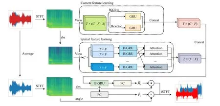
Fig.3.Overview of our SCGAD model architecture.A cube represents a tensor and a rectangle represents a learnable neural network layer.Meanwhile, layers of the same color indicate that they share parameters.

As a special case, whenQ,K, andVare of the same sequence, this mechanism is called self-attention mechanism,which has been widely used as a means of feature enhancement in various neural networks.

In order to use this mechanism more conveniently, we directly adopt two sub-network structures: Transformer encoder and Transformer decoder proposed by Vaswaniet al.[29],implemented by PyTorch [27].The proposed channel-compared attention is shown in Algorithm 1.

Algorithm 1 Channel-Compared Attention Forward Process Require: input spectrogram Y ∈RC×F×T X ∈RC×F×T Ensure: output spectrogram procedure FORWARD(X)for do φc=TransformerEncoder(F,n)c=1,...,C Init Φc=TransformerDecoder(F,n)Init uc=XT[c,...]∈RT×F uc=φ(uc)end for c=1,...,C for do c ＜C if then vc=XT[c+1,...]∈RT×F else vc=XT[0,...]∈RT×F end if wc=Φ(uc,vc)∈RT×F end for Y=concat(w1,...,wc)∈RC×T×F end procedure

D. Content Feature Learning

Since the model of treating the complex spectrogramX∈CC×F×Tas a complete sequence and using it in acoustic tasks has become relatively mature, we did not further motivate this task but directly adopted GRU.In this case, we treatXas a sequence of lengthTand hidden sizeC×F×2, and the hidden size is doubled since the real and imaginary parts of a complex are viewed as two separate parts.Fig.3 shows the complete model structure.

E. Loss Function

When designing the model, we still design the loss function from two perspectives: space and content, and propose a spatial-content loss (SCL) LSCL.First, to quantify the consistency of the content information, we use the L1 distance in both the time and frequency domains, as is common in source separation tasks [26], [28].Then, the core of LSCLlies in how to quantify the consistency of the spatial information.

The duplex theory provides the answer, i.e., ILD and ITD.However, ILD and ITD are not clearly defined mathematically.Although it is obvious for a single-source binaural signal (ILD can be obtained by comparing the amplitude of the peaks, and ITD can be obtained by comparing the position of the peaks), there are currently no good definitions of ILD or ITD for a multiple-source signal.

Therefore, we propose a compromise, that is, to treat the binaural signal as the sum of different frequency components and calculate the ILD or ITD for each component.Formally,for a given binaural signaly∈R2×L, we calculate the ILD ofyas

Then, for a predicted signalyˆ and the ground truthy, we can quantify the consistency ofILDas

For the ITD ofy, we can simply redefineMto ∠Yin (8).However, the angle operation will cause unstable training.Considering that ITD does not provide much information compared to ILD, as mentioned in Section III-B, we ignore ITD here.Finally, the proposed LSCLis defined as

It is worth mentioning that although our proposed LSCLdoes not consider ITD, we do consider ITD when evaluating the performance.The experimental results showed that our loss function can optimize ITD to a certain extent.

IV.EXPERIMENTAL SETUP AND RESULTS

In this section, we present the data collection process in Section IV-A and the experimental setup in Section IV-B.Our experiments can be divided into five parts:

1) We present an ablation study about proposed design ideas, which is shown in Section IV-C.

2) We present a performance study, which is shown in Section IV-D.

3) We present a hyperparameter sensitivity study, which is shown in Section IV-E.

4) We present a sample study that shows input and output spectrograms to further show the advantages of our method,which is shown in Section IV-F.

5) We present a blinded subjective study to supplement the above objective comparisons, which is shown in Section IVG.

A. Data Collection

To achieve end-to-end training, we developed and released a new dataset called the ByTeDance paired ambisonic and binaural (BTPAB) dataset1https://zenodo.org/record/7212795#.Y1XwROxBw-R.

The BTPAB dataset we released is based on a virtual concert scenario.Specifically, we recorded two musical performances in an anechoic chamber, one 31 minutes long for training and the other 18 minutes long for testing.To the best of our knowledge, it is the first dataset for comparing any endto-end deep models.Fig.4 shows our data collection environment.

The environmental sound recording equipment we used here was the H3-VR, while the binaural sound recording equipment was a Neumann KU100 dummy head.During the recording, we placed H3-VR on top of dummy head and recorded simultaneously.Unlike the traditional HRTF dataset,our data collection process is simple and effective.To better illustrate this point, we will further describe the details of the traditional HRTF dataset.

The format of the HRTF dataset is called the spatially-oriented format for acoustic (SOFA), which is a standard developed by the audio engineering society (AES).The SOFA format includes a matrix representing HRTFs and meta-informa-tion describing these HRTFs.Taking the HRTF dataset measured for the Neumann KU100 dummy head published by SADIE II [30] as an example, it includes: 1) An HRIR matrixH∈RM×R×N, whereM=1550 stands for 1550 different directions corresponding to HRIRs,R=2 stands for two ears andN=256stands for time impulse length.2) Meta information for describingH, such as the specific azimuth angleθ ∈RMand elevation angle Θ ∈RM, and the sample rater=48 000 of the time impulse.Such an HRTF dataset not only requires repeated measurement of HRTFs for thousands of directions,but also requires measurement in an anechoic chamber for accuracy reasons, and building an anechoic chamber is costly for general users.In contrast, the BTPAB dataset we publish here was collected in an anechoic chamber just for the sake of fair comparison rather than a necessary requirement.

In addition, HRTF datasets are difficult to use by end-to-end methods.Specifically, the goal of the spherical harmonicbased method is to mapHto another matrixHsp∈RD×R×Non the sphere based on spherical harmonic functions whereD=(n+1)2forn-order ambisonic.SinceD≪M, it is impossible to find a label that can be used for end-to-end training forHsp.

B. Settings

1)Training Settings: We first divide the 31-minute training audio into a group of non-overlapping 2-second segments, and feed every 16 segments as a batch to the model.After forward processing, we use the Adam optimizer [31] for backward processing with the learning ratelr=10-4and(β1,β2)=(0.9,0.009).Moreover, our training phase is divided into two stages: the first 10 000 updates are the warm-up stage[32], and the learning rate will increase linearly from 0 to 10-4.The second stage is the reduction stage.The minimum loss is checked every 1000 times to see if it has been updated.If not, the learning rate will be reduced by 0.9 times.

2)Evaluation Settings: The previous evaluation criterion cannot be directly used for the end-to-end methods since they are conducted on the HRTF dataset.Specifically,Hsp∈RD×R×Nis remapped back to the Cartesian coordinate system to obtainH′∈RM×R×N, and the difference betweenHandH′in magnitude and phase is compared as the evaluation criterion [6],[7], [9].

However, the comparison objects of end-to-end methods should be the predicted binaural signal and the ground truth.Therefore, we propose three criteria for the evaluation of endto-end methods from both spatial and content perspectives:

a)Content: We directly use signal-to-distortion ration(SDR) [33] to evaluate the content accuracy of predicted binaural signal.As a commonly-used indicator for measuring blind source separation, the SDR can reflect the numerical accuracy of the rendered signal.Formally, for a predicted signalyˆ ∈R2×Land the ground truthy∈R2×L, the SDR is defined as (unit: dB)

b)Spatial: According to duplex theory, we propose to evaluate the spatial accuracy from both ILD and ITD, although our loss function only considers ILD.

i)ILD: We propose the difference of interaural level difference (DILD), which is defined as (unit: dB)

whereILDis defined in (8).Note that the way we define ILD may have negative values, which means that the energy of the second channel is greater than that of the first channel.We then ignore the corresponding frequency components.To obtain more accurate results, DILD can be calculated by reversing ILD and calculating it again.

ii)ITD:We propose the difference of interaural time difference (DITD), which is defined as (unit: ms):

whereITDof a binaural signaly∈R2×Lis defined as

where “ ⋆” stands for cross-correlation operation andsrfor the sample rate ofy.

3)Model Settings: Our model has three hyperparameters:

a) The number of GRU layers denoted byL1.

b) The number of either Transformer encoder layers or Transformer decoder layers used in the proposed channelcompared attention mechanism.Here we useL2to denote both of them for simplicity.

c) The ratio of input feature dimensionality to output feature dimensionality of GRU layers, denoted byR.

We simply set bothL1andL2to 3 and setRto 1.Although our current setup does not achieve the best results on this dataset, it demonstrates that our method can handle this task well.Further parameter sensitivity study is shown in Section IV-E

C. Ablation Study

In Section III, we propose many design ideas.Here we will experimentally verify these ideas individually:

a)Feature representation

i) The proposed model uses a magnitude spectrogram to learn spatial features.Here, we set up two models for comparison.One model uses a complex spectrogram as input for spatial feature learning, denoted as “B”.The other model does not use spatial feature learning at all, denoted as “C”.

ii) The proposed model uses a complex spectrogram to learn spatial features.Here we set up two models for comparison.One model uses a magnitude spectrogram as input for content feature learning, denoted as “D”.The other model does not use content feature learning at all, denoted as “E”.

b)Spatial feature learning

i) The proposed model uses a channel-shared encoder for learning spatial features.Then, we set up one model for comparison, which adopts the general encoder design as [26], [28],denoted as “F”.

ii) The proposed model uses a channel-compared attention mechanism.Then, we set up one model for comparison, which disables the Attention mechanism, i.e., replacing the channelcompared Attention mechanism by an identity map, denoted by “G”.

c)Content feature learning: There is no comparative setting since we have not conducted more in-depth research on the content feature learning.

d)Loss function: The proposed model uses a spatial-content Loss during backward (L =Lspatial+Lcontent).Here, we set up one model for comparison, which uses Content Loss only (L =Lcontent), denoted by “H”.The reason why we did not conduct further experimental analysis on Lcontentis that the content loss we used is a mature design in the soundrelated field.

Table I shows our experimental ablation results.“Baseline”shows the existence of redefined ILD and ITD in binaural signals (DILD(yˆ,y)=ILD(y) sinceILD(yˆ)=0).Then, we can make the following analysis of the proposed design ideas:

a)Feature representation

i) By comparing to both “B” and “C”, we can claim that using magnitude spectrograms for spatial feature learning is useful (decreasing DITD from 0.66 or 0.63 to 0.52 and DILD from 10.11 to 9.65).Moreover, in our channel-compared design, using a complex spectrogram for spatial feature learning is insignificant.

ii) By comparing to both “D” and “E”, we can claim that using complex spectrograms for content feature learning is useful (increasing SDR from 6.30 or 6.51 to 8.30).“D” further shows that using only the magnitude spectrogram without considering the phase is not enough, which also agrees with Zhao’s claim [34].

b)Spatial feature learning

i) Compared to “F”, we can claim that using a channelshared encoder is more effective than a general encoder.“F”used more parameters and computation but performed worse on all metrics.

ii) Through the comparison to “G”, we can claim that using the channel-compared Attention mechanism is useful.

c)Loss function: Through the comparison to “H”, we canclaim that our proposed LSCLis useful for all metrics, especially for DILD (decreasing from 10.88 to 9.65).

TABLE I ABLATION STUDY OF PROPOSED MODEL ON BTPAB.SL.AND CL.MEAN SPATIAL FEATURE LEARNING AND CONTENT FEATURE LEARNING RESPECTIVELY, WHILE COM.AND MAG.MEAN THE COMPLEX AND MAGNITUDE SPECTROGRAM RESPECTIVELY.THE SETTING “BASELINE” SIMPLY AVERAGES THE VALUE OF INPUT ALONG THE CHANNEL AXIS TO GET A SINGLE CHANNEL AS BOTH LEFT AND RIGHT CHANNELS

TABLE II PERFORMANCE ANALYSIS OF PROPOSED MODEL ON BTPAB.THE SYMBOL “-”MEANS THAT NO RELEVANT STATISTICS HAVE BEEN CONDUCTED

D. Performance Study

In this paper, we propose the first end-to-end method for the binaural rendering of ambisonic signals.Here we present a comparative performance study with three traditional state-ofart baselines (SOTAs) and two end-to-end SOTAs from two different but similar tasks.These SOTAs are as follows:

a)Traditional

i) MagLS [6] (magnitude least square) which considers ILD.

ii) TA [7] (time-alignment) which considers ITD.

iii) BiMagLS (bilateral MagLS) which consides both ILD and ITD.

b)End-to-end

i) KBNet [35] from image denoising.

ii) MossFormer [36] form speech separation.

Table II shows our performance study.Then we can make the following analysis:

a)Traditional: All traditional methods have limited and similar performance on the proposed metrics.Traditional methods essentially compress HRTFs measured at multiple positions and frequencies (1550 and 256 respectively in our case) into spherical HRTFs that match the order of ambisonic signals (4 in our case).Therefore, the loss of accuracy is inevitable.The difference between different methods lies only in where the loss of accuracy occurs.When the criteria are blind to positions and frequencies, the difference between different methods is thus insignificant.

b)End-to-end

i) KBNet [35] cannot handle the binaural rendering well.A possible explanation is that the difference in inductive bias between images and the spectrogram of sounds is large.The performance of MossFormer [36] also supports this explanation.

ii) End-to-end methods are generally better than traditional step-by-step methods.Moreover, our method performs better than other methods that are not designed specifically for spatial information.

E. Sensitivity Study

We conduct sensitivity experiments for two parameters.One is the number of learnable layers, including the number of GRU layers and the number of encoder and decoder layers used in the attention mechanism.The other is the ratio of input feature dimensionality to output feature dimensionality for learnable layers if possible.

Table III shows the sensitivity experiment for the number of learnable layers.For simplicity, we set the number of GRU layers equal to the number of encoder and decoder layers used in the attention mechanism.The experiment showed that too many layers ( ＞4) would make it difficult for the model to converge.Based on the performance, we believe that choosing 3 as the number of learnable layers is reasonable.

Table IV shows the sensitivity experiment regarding the ratio of input feature dimensionality to output feature dimen-sionality of a single learnable layer.Since the Attention API provided by PyTorch [27] does not change the dimensionality and the output feature dimensionality of the used DNN is fixed (same as the ground truth binaural signals), our experimental settings only affect all GRU layers.In order to avoid an OOM (out of memory) issue, we change the batch size for the experiment corresponding to a ratio of 1.25.Although using higher dimensionalities can improve the performance of the model, especially DITD, the increased cost is unacceptable.We still recommend using a ratio of 1.

TABLE III LAYER NUMBER SENSITIVITY ANALYSIS OF PROPOSED MODEL ON BTPAB.THE SYMBOL “-”MEANS THAT THE CORRESPONDING MODEL IS NOT CONVERGED

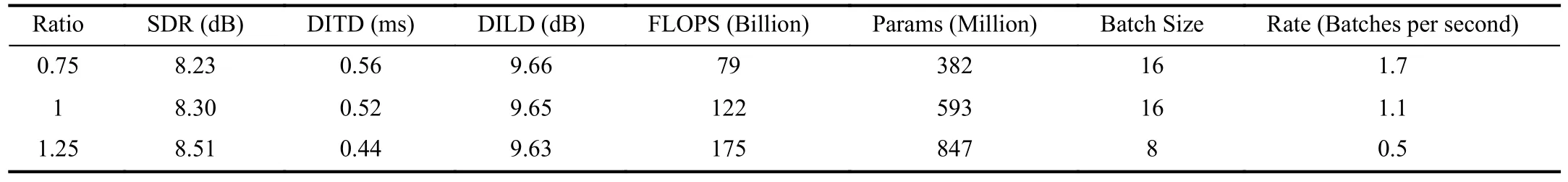
TABLE IV DIMENSIONALITY RATIO SENSITIVITY ANALYSIS OF PROPOSED MODEL ON BTPAB

F. Sample Study

We further present the results in detail in Fig.5 when the input is a slice of the test ambisonic audio, and the details of the input are shown in Fig.2.

From the second row of Fig.5(a), we can see that there are two obvious problems with MagLS [6] on SADIE II [30]:

1) The overall energy level is higher than expected.

2) There are many high-frequency components that should not exist.

We believe that those extra high-frequency components stem from the low frequency resolution of the HRTF dataset.Specifically, the HRIR of the dataset we used has 256 sampling points at a sampling rate of 48 000 Hz.On the other hand, the overall energy level is due to the error of the algorithm.

To further demonstrate the numerical accuracy challenge,we show the ILD in the second row of Fig.5(b).There are also two issues here:

1) In the time domain, it loses the blank band near the 500th frame.

2) In the frequency domain, it loses two more obvious blank bands located roughly at the 280th and 600th frequency bins,and a less obvious blank band located roughly at the 30th frequency bin.

We believe this is mainly because MagLS does not consider the interference between multiple sound sources in space.However, this is also a common problem with previous methods.

We show our result in the third row of Figs.5(a) and 5(b).From the perspective of the magnitude spectrogram, we have maintained a good level of energy, and there are no additional frequency components.However, our result has lost some detailed information, although it may not sound obvious.We believe that this is due to the overly simple model structure used in content feature learning.On the other hand, from the perspective of the DILD, our result has better maintained key patterns.

G. Blinded Subject Study

We recruited eight volunteers from a local university for subjective study.We randomly selected 20 s of the ambisonic signal from the test dataset as input, and then had volunteers listen to the corresponding binaural signal.Finally, we had volunteers listen to the outputs of all settings mentioned (“A”to “H” in Section IV-C) in the ablation study.Those settings are blind to the volunteers.

Since our volunteers are not professionals, using mean opinion score (MOS) will introduce considerable randomness.Therefore, we organized a questionnaire survey and asked the following questions:

1) Which audio is most similar to the ground truth (the responding binaural signal)?

2) Can you hear the spatial information in the ground truth,such as the approximate orientation of instruments and vocals in space (It is to screen out volunteers who can represent the head model used when recording the dataset)

3) Can you sense the spatial information in these output audios?

4) Which audio is closest to the ground truth in terms of spatial information?

5) Which audio is the worst in terms of both spatial information and listening experience?

From the feedback, “A” is clearly similar to the ground truth.All volunteers said that they can hardly discern the difference between “A” and the ground truth.Meanwhile, “D”and “E” are the worst, with 3 and 5 votes, respectively.Volunteers said that the difference in the spatial information is not obvious, and the reason why they are the worst is that they sound dull and lack detail.This indicates that learning of content features is necessary.

Fig.5.Sample study of the 240 s to 260 s of the test ambisonic audio.(a) Shows the output magnitude spectrograms.Two columns corresponds to left-channel and right-channel, respectively (b) Shows the output DILDs calculated in (14).From top to bottom of both (a) and (b), we show the ground truth, result predicted by MagLS [6] on SADIE II [30] and our SCGAD result.

In addition, we also had volunteers listen to the output of MagLS [6].Volunteers feedback that it sounds fine but dissimilar to the ground truth.Specifically, volunteers said that it seems to be recorded in a narrower place, and the difference in relative position between instruments and vocals in the longitudinal direction is much smaller.

V.DISCUSSION

We will discuss possible questions here.

A. Robustness

In this paper, as the first end-to-end method, we not only proposed a model architecture but also proposed a dataset.Therefore, we also need to consider robustness from two perspectives:

1) Can our model be applied to future datasets that may be released? Our answer is yes, for two reasons: a) The dataset we evaluated corresponds to a rather complex scenario, and our model can perform well.b) It is unlikely that there will be a dataset in the future that contains data from many different sound scenes.This is because the dynamic systems in different sound scenes are different.For example, the sound propagation process in indoor and outdoor environments is different.Therefore, it is more practical for a dataset to contain only one or one type of sound scene.

2) What is the representational power of our dataset for the real world? Our answer is limited.Real-world scenarios are complex, and this complexity is reflected in two aspects.One is the dynamic system of the sound field, including the types and positions of sound sources, propagation media and reverberation.The other is the propagation process of sound to the human ear, including the relative position of people in the sound field and the shape of human ears.Our dataset can only represent one type of sound scene, but is sufficient to verify the effectiveness of our method.

B. Usefulness

For this task, it is unlikely that there will be a dataset with strong expressive ability, and this is precisely where the value of our method lies.Because users are likely to need to record additional datasets for their use cases, and our method only needs to record for approximately 30 min in a specific sound environment to achieve good results.

In addition, we provide more of an idea, and users can easily expand it according to their actual situations.For example,we can use other more complex Encoders to replace the GRU in our model to achieve better results, or use simpler Attention mechanisms to replace the PyTorch API we used when there are hardware limitations.

C. Future: Universal Model

A universal model for multi-individual situations is of great research value.Due to the limitations of this task, the input must include the physical information of individuals, and the encoding of physical information is challenging.Previously,the encoding process was implicitly included in the HRTF measurement.However, for end-to-end methods, it is inappropriate to use HRTF as a part of the input, since HRTF is not accurate enough while a large number of parameters (1550 ×2 × 256 in SADIE II [30]) are used.Based on existing related works [37], [38], we believe that there are two choices.

The first is to use photos of the pinna.The advantage is that it is convenient for users, but the disadvantage is that it is difficult for dataset collection and model design.Because the dataset needs to include multiple photos of the same person to ensure robustness, the model would require a special module to further learn the characteristics of people based on photos.The second choice is to directly transmit the physical information of the head through point clouds or other modelling methods.This approach is not convenient for users, but it is beneficial for model design because these point clouds are relatively accurate.

VI.CONCLUSION

In this paper, we propose a novel end-to-end ambisonic-binaural audio rendering approach by simultaneously considering spatial feature and content feature.Considering that general acoustic tasks do not take into account the spatial feature of sound, we propose some improvements on the spatial information of sound based on using traditional network structures to learn the content features of sound.Specifically, we propose to learn spatial features of sound by combining channelshared Encoder and channel-compared attention mechanism.

To verify the effectiveness of proposed method, we collect a new ambisonic-binaural dataset for evaluating the performance of deep-learning-based models, which has not been studied in literature.Then, we propose three metrics for evaluating end-to-end methods, including: 1) SDR, which measures the consistency of content information, 2) DITD, and 3)DILD, which measures the consistency of spatial information.Experiments show the promising results of the proposed approach.In addition, we demonstrate and analyze the shortcomings of the traditional methods.

Although our experimental results show that the proposed spatial-content decoupled network design is effective, there are still shortcomings.Firstly, on learning spatial features, the attention mechanism we use brings a large number of parameters and computations, and future work can study how to use a more effective way to compare different channels to learn spatial features.Secondly, on learning content features, we directly use a relatively simple structure in our proposed method without further optimization, which leads to the loss of some details in our results.In the future, we will focus on how to further optimize the learning process of content features.