Temperature field test and prediction using a GA-BP neural network for CRTS II slab tracks
Dan Liu · Chengguang Su · Rongshan Yang · Juanjuan Ren · Xueyi Liu
Abstract The CRTS II slab track, which is connected in a longitudinal direction, is one of the main ballastless tracks in China, with approximately 7365 km of operational track.Temperature loading is a very vital factor leading to slab track damages such as warping and cracking.While existing research on temperature distribution rests on either site tests in special environments or theoretical analysis, the long-term temperature field characteristics are not clear.Therefore, a long-term temperature field test for the CRTS II slab track on bridge-subgrade transition section was conducted to analyze the temperature field.A GA-BP(genetic algorithm optimized back propagation) neural network was trained on the test data to predict the temperature field.The vertical and lateral temperature distributions in four typical days were carried out.We found that the temperature along the track was distributed in a nonlinear manner.This was particularly distinct in the vertical direction for depths of less than 300 mm.The highest and lowest daily temperatures and the daily range of the temperature were analyzed.With the increasing depth, the daily highest temperatures and range of the temperature were smaller, the daily lowest temperatures were higher,and the time corresponding to this peak value appeared later in the day.Both the highest and lowest daily temperature could be predicted using the GA-BP neural network, though the accuracy in predicting the highest temperature was higher than that in predicting the lowest temperature.
Keywords Ballastless track · Long-term test · Temperature distribution · Correlation analysis · Neural network
1 Introduction
Ballastless tracks, which are characterized by good smoothness, high reliability and low maintenance requirements,have long been used as the main track structure on China’s high-speed railways [1, 2].The CRTS II slab track is one of the main ballastless tracks in China and has been successfully applied on 7362 km including the Beijing-Tianjin Intercity Railway and Beijing-Shanghai High-Speed Railway.In addition to withstanding train loads, the ballastless track must also be able to resist temperature loads caused by solar radiation, atmospheric temperature, wind speed and other meteorological factors [3].Due to the poor thermal conductivity of reinforced concrete, these complex meteorological effects may cause uneven temperature distribution in the track slab, leading to considerable temperature stress.This will ultimately lead to slab track damage such as warping, cracking and other irregularities [4-8].Therefore, a temperature field analysis is of great significance for improving durability and ensuring operating safety.
In recent years, specific models have been proposed to analyze the temperature distribution on a ballastless track.Zhang et al.[9] built a refined spatial finite element model for continuously welded rails (CWRS) on the CRTS II slab tracks of a long-span bridge, and found that the transverse temperature gradient of the track slab had a significant effect on the stress and displacement of both track and bridge.According to solar radiation and boundary heat transfer theories, Zeng et al.[10] established a temperature field analysis model to explore the influence of alignment and geographical latitude on the temperature distribution of ballastless track.Utilizing a spectral analysis of meteorological parameters and measured temperature, Yang et al.[11] established a theoretical prediction formula to analyze the influence of meteorological parameters on the temperature field of ballastless track, and acquired the associated temperature distribution under extreme heat.Zhou et al.[12]built a transient model to analyze the effect of wind speed and solar radiation intensity on the temperature distribution of the CRTS III slab track.Zhang [13] analyzed the time distribution characteristics of surface temperature, along with the temperature gradient of ballastless track in different areas, and found that there is a strong linear correlation between the surface temperature and the environmental temperature.Based on a correlation analysis, the accuracy of the BP neural network and the LSTM neural network model could be compared.
Many studies have also focused on temperature distribution tests for ballastless track.Lou et al.[14] investigated the temperature action of a China’s HSR bridge-track structure based on one year of observational data and predicted the extreme temperatures of the track-bridge system.Dai et al.[15] studied the vertical and transverse temperature load based on a CRTS II slab track field test and proposed that the maximum temperature change of the track slab surface was 15 °C.Zhao et al.[16] conducted a series of temperature distribution tests on CRTS II ballasted track on a bridge in summer using a 1:4 scale model and showed that vertical temperature shows an s-shaped nonlinear distribution.The transverse temperature distribution obtained in this way was a parabolic curve, and the three-dimensional temperature distribution was a saddle-shaped surface.Zhou et al.[17] conducted a 1/4 scale model test to analyze the temperature field distribution of the CRTS II slab track on a bridge under rapid temperature fluctuations, and put forward a three-dimensional distribution pattern for the transverse and vertical temperature of the track system.Yang et al.[18] monitored the temperature distribution of the CRTS twin-block track in winter, obtaining a vertical temperature load model by means of mathematical statistics.
The above research on temperature distribution was all based on site tests in special environments, such as during extreme heat or winter, or based on theoretical analysis.However, daily environmental temperature changes are never uniform, and precise temperature distribution rules are diffi-cult to explore, meaning that there is also a need for in-depth monitoring and analysis of long-term temperature distribution data on ballastless tracks [19].In this work, a one-year temperature field monitoring test was conducted on CTRS II continuous ballastless track installed on the Shanghai-Hangzhou high-speed railway.The temperature field distribution,along with daily highest and lowest temperatures and their occurrence time, was analyzed with monitored data from different seasons.Temperature was then predicted using GA-BP neural networks.
2 Description of field experiment
2.1 Investigation of the test site
East China has a subtropical monsoon climate with welldefined seasons.It is a good area for monitoring and analyzing variations in temperature fields.For this reason, the bridge-subgrade transition section of the Haining maintenance area on the Shanghai-Hangzhou high-speed railway was chosen as a suitable test site.The tested structure was the CRTS II slab track, which is connected in a longitudinal direction [20].As shown in Fig.1, this test site features good ventilation, a wide angle of vision and no shelter from large structures, and receives significant amounts of sunshine.This is in line with the requirements for monitoring meteorological factors such as air temperature, solar radiation,wind speed, etc.Moreover, the maintenance area can provide power for the testing facilities, and is a suitable location for placing monitoring equipment, making it the ideal location to monitor the temperature field within the ballastless track.

Fig.1 Test site: a layout of test site; b tested track
2.2 Monitoring set-up
In this test, the temperature field data for the ballastless track was tested, along with meteorological data.The specific monitoring data obtained was as follows:
(1) The temperature of the ballastless track, which included the temperature of the track slab, concrete roadbed, and subgrade;
(2) Meteorological parameters, including air temperature,solar radiation intensity, wind speed, precipitation,humidity, and other weather data.
Based on existing research on temperature change and transfer characteristics of ballastless tracks [21], the track slab shows a greater sensitivity to meteorological factors than other components do, meaning that more sensors are required to analyze its temperature field.The CRTS II slab track is continuous in the longitudinal direction, meaning that the longitudinal temperature remains at a relatively constant level.Using only one cross section (see Fig.2), it is therefore possible to obtain effective temperature field data.In this test, 13 thermal sensors (1-1-1-13) were installed in one cross section to measure the vertical temperature distribution (see Fig.2a).For the track slab and concrete roadbed, there were 6 sensors each, and the space between two adjacent sensors was 40 and 60 mm, respectively.Because the mortar adjustment layer was only 30 mm in height, and the sensors at the track slab bottom and the top of the concrete roadbed had intruded into the mortar layer, so we didn’t install sensors in this layer.There was one sensor installed at the center of the subgrade.Based on existing research,the lateral temperature was uniformly distributed in the central area, which was located 400 mm away from the slab edge.So there was only one thermal sensor (1-4) in the central area, and 4 thermal sensors (1-14-1-17) were in the edge area.All lateral thermal sensors were laid at a depth of 120 mm away from the top of the track slab (see Fig.2b).
Since the track structure was already installed before testing, thermal sensors were placed within a prefabricated concrete pillar.First, the concrete was poured into a steel pillar mold with 13 holes, and all holes were sealed up with adhesive tape.Before the initial concrete was set, adhesive tape was ripped offand temperature sensors were inserted into those holes.After 28 days of curing, the mold was removed,and the pillar is shown in Fig.3.A 30 mm diameter hole was then drilled in the middle of the slab track.After drilling,the hole was cleaned and dried with a blower.Finally, the prefabricated concrete pillar was inserted into the hole and the DG-BMT poured into it in order to bond the pillar with the slab track, as shown in Fig.4.

Fig.2 Thermal sensor distribution in the CRTS II slab track (unit: mm): a vertical distribution; b lateral distribution

Fig.3 Prefabricated pillar with sensors

Fig.4 Photograph of the test site
2.3 Testing apparatus
A PT100 platinum thermal resistance sensor, featuring an anti-vibration and anti-corrosion probe, and exhibiting excellent high temperature and pressure performances, was used for this test.The high-precision platinum resistance element within this sensor is able to measure temperatures more accurately and reliably than other products.An intelligent high-speed itinerant static strain data acquisition system-DH3821 was used to acquire the corresponding data.As shown in Fig.5, the remote monitoring system consisted of an industrial personal computer and a 3G wireless communication system.
3 Temperature distribution on ballastless track
3.1 Vertical temperature distribution
The vertical temperature distributions on the track on four typical days across seasons are shown in Fig.6.In general, it can be seen from Fig.6 that the temperature was nonlinearly distributed.As depth increased, the temperature change gradually slowed down, and the daily temperature amplitude variations decreased.Especially for a depth of less than 300 mm,the nonlinear features were very distinct.For depths greater than 300 mm but less than 550 mm, the temperature changed linearly with depth.For depths greater than 550 mm, the temperature remained fairly constant, suggesting environmental factors had little impact on the temperature within the track.For the track slab, the maximum vertical temperature difference between the top and bottom reached about 12 °C.

Fig.5 Remote monitoring system
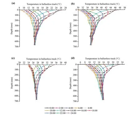
Fig.6 Temperature in ballastless track at different depths: a Mar.8 in spring; b Aug.15 in summer; c Oct.1 in autumn; d Dec.8 in winter
As Fig.6 shows, the temperature at the top of the track slab indicates the largest variation in amplitude.Since the top was directly exposed to the environment, it can easily engage in heat exchange.As the depth increased, the heat transfer rate between the track and the environment decreased, showing that environmental influence had also become less pronounced.
At the same depth from the slab track top, the temperature and its daily amplitude varied across seasons.In spring and summer, the daily temperature variation amplitudes for the track slab at the top were the largest, while in autumn it was the smallest.From Fig.6, it can be found that in the four typical days, the temperature gradient in the track slab was positive from 8:00 to 16:00.From 18:00, the temperature started to fall, and the temperature gradient became negative.However, the negative temperature gradient and temperate fall rate in spring and summer were larger than those in autumn and winter.
3.2 Lateral temperature distribution
Figure 7 shows the temperature lateral distribution of the ballastless track on 4 typical days in the different seasons.From Fig.7, it is clear that the lateral temperature distribution in the ballastless track was not uniform.The temperature lateral distribution can be divided into two parts, the first part is the central area about 975 mm away from the center, and the second part is the edge area.In the central area, with the increase of lateral distance, the temperature always slightly decreased.For the edge area, the temperature decreased with the increase of the lateral distance from 20:00 to 8:00, and it increased as the lateral distance from the center increased from 08:00 to 20:00 in winter, while it increased from 10:00 to 20:00 in other seasons.In general,temperatures changed uniformly in the central area, while in the edge area, the variations of temperature were different from the lateral distance.It can be found that the edge area tended to be more influenced by the environment.But compared with the vertical temperature gradient, the lateral temperature gradient was much less.The maximum lateral temperature difference was about 2 °C.

Fig.7 The temperature in ballastless track at a different lateral distance: a Mar.8 in spring; b Aug.15 in summer; c Oct.1 in autumn; d Dec.8 in winter
4 Highest daily temperatures in ballastless track
4.1 Highest daily temperature
Comparing the environmental temperature and the temperature of the ballastless track (see Fig.8), it can be seen that like the environmental temperature, the daily highest temperature on the track structure also exhibited a sinusoidal trend with the date.The highest temperature on the track structure fell to a minimum in January or February and rose to a maximum in August.It can be seen that the highest daily temperature of the track slab displayed significant seasonal variations, and that with an increase in environmental temperature, the highest daily temperature became even higher.
As shown in Fig.8, the highest daily temperatures measured at the top of the track slab were the largest, and were always greater than the environmental temperature.From the top of the track slab to the center of the concrete roadbed,this temperature then decreased as the depth from the top increased, with both being larger than the environmental temperature.From the center of the roadbed to the subgrade,the highest daily temperature almost remained at the same level from the center to the bottom, with some being lower than the environmental temperature.
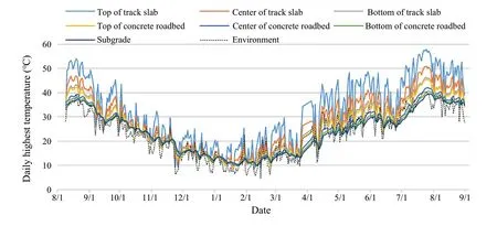
Fig.8 Highest daily temperature throughout the year
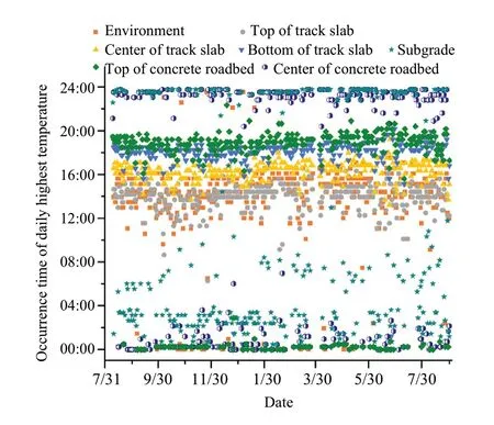
Fig.9 Occurrence of the highest daily temperature
4.2 Time of highest daily temperature
Figure 9 indicates the time at which the highest daily temperatures occurred.It is clear that the temperature at the top of the track slab reached its highest value earliest, being close to the time that the highest daily environmental temperatures occurred on many days.With increasing depth from the top, the time that the highest temperature occurred became later in the day.On most days, the temperature at the top of the slab track reached its highest value at about 13:00-15:00, and the center of the slab track reached its highest temperature at 15:00-17:00, while the bottom of the track slab and top of the concrete roadbed reached this temperature later, which was at 18:00-20:00.The times that the highest temperature occurred in the concrete roadbed center and subgrade were obviously later and discrete, which is about 22:00-04:00.Sometimes, however, the highest daily temperature occurred at about 0:00.When compared with the meteorological data, it was found that there had been a continuous reduction in air temperature during these days.Data for the highest daily temperature lag time between the track slab and the environment are shown in Fig.10.It was observed that the time of highest daily temperature at the top of the track slab occurred close to that of the environmental temperature, with a mean lag time of about - 0.204 h,while that of the track slab center significantly lagged behind the environment, with a mean lag time of 0.644 h.As the depth increased to the bottom of the track slab, a further increase in lag time could be found, the upper and lower quartiles were both larger.As the depth decreased to the top of the concrete roadbed, the mean lag time increased to 0.76 h.For the concrete roadbed center and subgrade, the boxes of lag time were longer than others, they had bigger upper quartiles and smaller lower quartiles.This implies that the moments of the highest temperature were more discrete.
4.3 Correlation analysis
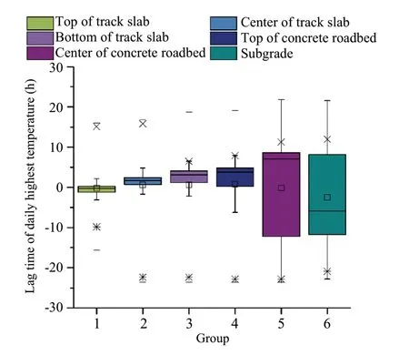
Fig.10 Boxplot for lag time of the highest daily temperature between track slab and environment (-means max and minimum value, × means 99% value, and * means 1% value)
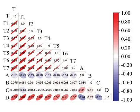
Fig.11 Pearson correlation coefficients for highest daily temperature in slab track, and other meteorological parameters (T is the environmental temperature, A the humidity, B the daily maximum wind velocity, C the daily precipitation, and D the daily solar intensity)
To find the relationship between the highest daily temperature in the track slab and the meteorological parameters, the correlation coefficients were taken out as shown in Fig.11, where T1-T3 are the highest daily temperatures at the top of the track slab,center, and bottom, respectively.T4-T6 represents the highest daily temperature at the top of the concrete roadbed center,and bottom, respectively.While T7 represents the highest daily temperature of the subgrade.T is the highest daily environmental temperature.A-D are the meteorological parameters.From Fig.11, it can be seen that the highest daily temperature in the track slab had a significant positive correlation with both environmental temperature and daily solar intensity, but a negative correlation with humidity.The highest daily temperature in the slab track showed the strongest correlation with the highest daily environmental temperature, ranging from 0.92 to 0.98.With increasing depth, the correlation coefficients of the highest daily temperature in the slab track with the highest daily environmental temperature gradually decreased, except for those located at the top of the track slab.The correlation coefficient of the highest daily temperature at the top of the track slab with the highest daily environmental temperature was slightly less than that in the track slab center.This could potentially be because the top of the track slab is more likely to be affected by other meteorological factors.The correlation coefficients of the highest daily temperature in the slab track with daily solar intensity ranged from 0.50 to 0.82, and decreased as depth increased.In general, the highest daily environmental temperature had the greatest impact on the highest daily temperature in the slab track,while the daily solar intensity also had a significant impact on the highest daily temperature in the slab track.The humidity had a slightly negative impact, while wind velocity and daily precipitation barely had any noticeable impact at all.
5 Lowest daily temperatures in ballastless track
5.1 Lowest daily temperature
Figure 12 indicates the lowest daily temperatures in the ballastless track.It was also found that the temperature trend for the track slab was similar to that of the surrounding environment, and that the lowest daily temperature of the track slab was still higher than that of the environment.Among these,the lowest daily temperature at the top of the track slab was close to that of the ambient temperature.From the top to the center of the track slab, the lowest daily temperature increased as the depth increased.From the bottom of the track slab to the subgrade, the lowest daily temperature at different depths remained almost the same.Compared with the highest daily temperature, it was clear that the lowest daily temperature difference between the track slab and the environment was much less significant.
5.2 Time of lowest daily temperature occurrence

Fig.12 Lowest daily temperatures throughout the year
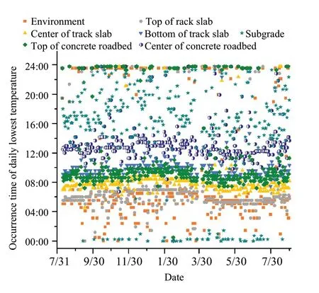
Fig.13 Time of occurrence of the lowest daily temperature
The times that the lowest daily temperature occurred are shown in Fig.13, with the lag time of lowest daily temperature between track slab and environment shown in Fig.14.It can be seen that the top of the track slab reached its lowest daily temperature at around 06:00, and that this time was similar to that of the environmental temperature.The distribution of lag time between the top of the track slab and the environment was more concentrated, with upper and lower quartiles of 0.72 and - 0.24 h, and a mean value of only - 0.133 h.When the depth from the top increased, the moment the lowest daily temperature occurred appeared later in the day and the lag time became more discrete, especially for depths increased to the center of the concrete roadbed.For the track slab center,it reached its daily lowest temperature at 07:00-09:00, the upper and lower quartiles lag times were 2.91 and 1.23 h,respectively, with a mean value of 1.022 h.For the track slab bottom and concrete roadbed, they reached their daily lowest temperature at 08:00-10:00, and their mean lag times were 1.809 and 2.405 h, respectively.The upper and lower quartiles of the concrete roadbed center were much larger than those of the concrete roadbed top, with a mean time of 4.97 h.For the subgrade, the degree of discretization of the lag time of the sublattice was more pronounced.From Fig.13, it can be seen that there were a few days when the lowest daily temperature occurred at about 00:00.When compared with the meteorological data for that period, it was found that the environmental temperature had been increasing continuously at that time.

Fig.14 Boxplot of lag time for the lowest daily temperature between track slabs and environment
5.3 Correlation analysis

Fig.15 Pearson correlation coefficients for the lowest daily temperature in slab tracks and meteorological parameters
The correlation coefficients between the lowest daily temperature and meteorological parameters are indicated in Fig.15.T′1-T′3 are the lowest daily temperatures at the top of the track slab, the center, and the bottom, respectively.T′4-T′6 represent the lowest daily temperatures at the top of the concrete roadbed, the center, and the bottom, respectively.T′7 represents the lowest daily temperatures in the subgrade.T′is the lowest daily environmental temperature.Meteorological parameters A-D are the same as in Fig.11.From Fig.15, it can be seen that environmental temperature has the greatest influence on the lowest daily temperature of the track slab, where the correlation coefficient was as high as 0.99.Even for the subgrade, the correlation coefficient was 0.96.Meanwhile, D (daily solar intensity) has a significant effect on the lowest daily temperature of the ballastless track, with the correlation coefficient going up to 0.52, though this was much smaller than that of the highest daily temperature.A(humidity) slightly affected the lowest daily temperature of the track with a negative correlation coefficient of 0.16, though since their correlation coefficients were less than 0.1, it can be seen that B (wind velocity) and C (daily precipitation) barely affected the lowest daily temperature at all.
6 Daily range of the temperature
6.1 Daily range of the temperature
The daily range of the temperature for the ballastless track are shown in Fig.16, and their statistical characteristics are shown in Fig.17.It can be found that the daily range of the temperature at the top of the track slab was the largest,and was even always larger than that of the environment.The mean daily range of the temperature at the top of the track slab was 13.09 °C, while that of the environment was 7.50 °C.With increasing depth from the top, the daily range of the temperature decreased, but the decrease rate became moderate as the depth increased towards the center of the concrete roadbed.From the top of the track slab to the center of the concrete roadbed, the mean daily range of the temperature decreased from 13.09 to 0.925 °C, and this value of the subgrade was 0.737 °C.As shown in Fig.15, the daily range of the temperature varied across seasons, in autumn and winter they were much smaller than those in spring and summer,especially for the track slab and the upper half of the concrete roadbed.The largest daily range of the temperature at the top of the track slab reached 25.81 °C in June, and the smallest was 0.453 °C in Jan.With increasing depth from the top,the box in Fig.17 was shorter, and the annual variation was less.For the center of the concrete roadbed and subgrade,the maximum daily range of the temperature was 2.467 and 2.03 °C, respectively, and the minimum daily range of the temperature was 0.051 and 0.042 °C, respectively.
6.2 Correlation analysis

Fig.16 Daily range of the temperature throughout the year
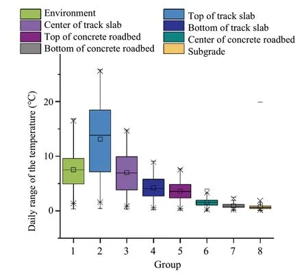
Fig.17 Boxplot of the daily range of the temperature throughout the year
Figure 18 indicates the correlation coefficients between the daily range of the temperature and meteorological parameters.ΔT1-ΔT3 are the daily range of the temperature at the top of the track slab, the center, and the bottom, respectively.ΔT4-ΔT6 represent the daily range of the temperature at the top of the concrete roadbed, the center, and the bottom, respectively.ΔT7 represents the lowest daily range of the temperature in the subgrade.ΔT is the daily range of the environmental temperature.Meteorological parameters A-D are the same as in Fig.11.From Fig.18, it can be seen that the daily ranges of the temperature had obvious positive correlations with the daily solar intensity and environmental daily temperature difference, but negative correlations with the humidity and daily precipitation.Unlike the daily highest or lowest temperature, the daily solar intensity was the most strongly correlated factor, and the daily precipitation became a significant effect.For the top of the track slab, the correlation coefficient of the daily ranges of the temperature with the daily solar density and the environmental temperature difference were 0.95 and 0.85, respectively, while the correlation coefficients with the humidity and daily precipitation were - 0.40 and - 0.35, respectively.With increasing depths, the daily ranges of the temperature became less relevant to meteorological parameters.For the subgrade, the meteorological parameters barely had an influence on the daily ranges of the temperature.
7 Temperature prediction based on GA-BP neural networks
7.1 GA-BP neural network model
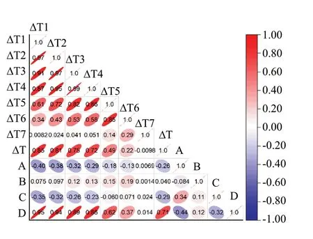
Fig.18 Pearson correlation coefficients for daily ranges of the temperature in slab track and other meteorological parameters
The BP neural network has good nonlinearity and flexibility, can learn and store a lot of mapping relations of input and output modes and needn’t to describe the mathematical equation of the mapping relation.It is composed of an input layer, an output layer and several hidden layers, and is a form of guided learning algorithm [22].During forward propagation, the neurons within each layer only affect the subsequent layer.When there are errors between the actual output and the expected output, the BP neural network starts a process of back-propagation, which is a means of correcting the connection weight between different levels.Iteration via forward and backward propagation enables errors to be minimized.The BP neural network has been successfully used for predictions in many fields [23, 24].However, due to the randomness of the initial connection weights and thresholds, it often leads to unreliable output values.Genetic algorithm (GA) can be searched globally when solving the model, and can ensure the global optimal solution according to the convergence in a short time.The GA and BP can be complementary.Using genetic algorithms to optimize connection weights and thresholds is an effective way of compensating for this deficiency[25].The GA-BP model not only has the nonlinear mapping ability of BP network, but also has the global optimization search capability of genetic algorithm.Therefore, a set of GA-BP neural networks were designed in MATLAB and used to predict the temperature of the CRTS II track slab.
A little after this the princess said again to the prince, Look round; do you see anything behind us? Yes, said the prince, the big black cloud is there again
Among the 378 sets of monitoring data collected over a year, 80% of the data was randomly selected to train the neural networks, while the rest of the data was used to validate it.There were 5 groups of input vectors: environmental temperature, humidity, daily maximum wind velocity, daily precipitation and daily solar intensity, and one output vector: highest (lowest) daily temperature.Due to the different orders of magnitude within the sample data, which could affect identification accuracy, all data was normalized using the following Eq.(1).
wherex′is the normalized output of the parameterx,xmaxis the maximum value of the parameterx, andxminis the minimum value of the parameterx.
In this GA-BP temperature prediction neural network model, the initial population size was 30, the maximum genetic generation was 50, the crossover probability was 0.8, and the mutation probability was 0.2.The Levenberg-Marquard algorithm was used to train the network.The optimal number of hidden layer nodes (hn) was determined by means of the following equation:
wheremis the number of neurons in the input layer,nis the number in the output layer, andais an integer ranging from 1 to 10.By training the BP neural network with a traversing value of a from 1 to 10, the optimal hidden layer node number can be obtained.
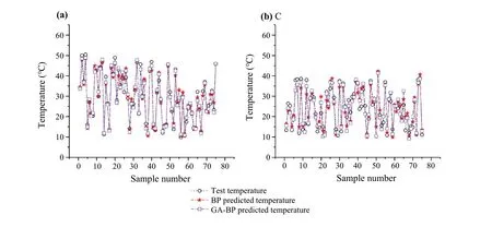
Fig.19 Predicted results for the highest daily temperature: a track slab; b concrete roadbed
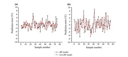
Fig.20 Absolute error for the highest daily temperature: a track slab; b concrete roadbed

Table 1 Comparisons of the highest daily temperature error
7.2 Highest daily temperature prediction
The highest daily temperature prediction results and absolute errors are given in Figs.19 and 20, respectively.It can be seen that, when using monitoring data taken across a whole year,the GA-BP neural network is able to predict the highest daily temperature very accurately.Compared with the BP neural network, the GA-BP network can significantly reduce absolute errors.For the track slab, the maximum absolute error of the BP neural network and the GA-BP neural network were 6.42 and 5.01 °C, respectively.For the concrete roadbed, the maximum absolute errors were 9.00 and 7.29 °C.
The prediction errors for highest daily temperature are given in Table 1.After optimizing connection weights and thresholds using the genetic algorithm, the mean absolute error (MAE), root mean square error (RMSE), and mean absolute percentage error (MAPE) all decreased.It can therefore be concluded that the prediction accuracy was improved.For the track slab temperature predicted using the GA-BP model, the MAE and RMSE were 1.328 and 1.651 °C, respectively, while the MAPE was 5.040%; for the concrete roadbed temperature, the MAE and RMSE were 2.228 and 2.807 °C, while the MAPE was 11.053%.Because the highest daily temperature of the track slab is more sensitive to environmental influence, and since the correlation coefficients between the track slab temperature and the meteorological parameters are larger, BP-GA neural networks are able to provide better predictions for track slab temperature.
7.3 Lowest daily temperature
Prediction results and absolute errors for lowest daily temperature are described in Figs.21 and 22, respectively.From these figures, it can be seen that the lowest daily temperature can also be predicted using neural networks, and that the GA-BP neural network has better accuracy.The maximum absolute errors in lowest daily temperatures on the track slab and the concrete roadbed were - 11.29 and - 10.77 °C, which were larger than those of the highest daily temperature.

Fig.21 Predicted results for the lowest daily temperature: a track slab; b concrete roadbed
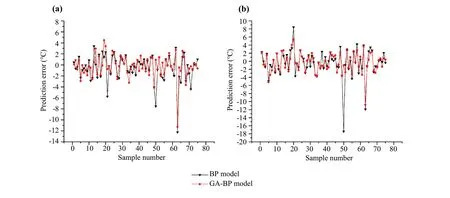
Fig.22 Absolute error for lowest daily temperature: a track slab; b concrete roadbed

Table 2 comparisons of the lowest daily temperature error
8 Conclusions
The temperature field for ballastless track on the Shanghai-Hangzhou High-Speed Railway was monitored for a whole year, during which time the vertical and lateral temperature distribution were analyzed.The daily highest and lowest temperatures at the top of the track slab were predicted by means of GA-BP neural networks.Conclusions can be drawn as follows:
(1) The temperature distribution along the track was nonlinear in form.In the vertical direction, and for depths less than 300 mm, this nonlinearity was particularly pronounced.With increasing depth, the rate of temperature change gradually decreased, and the amplitude of daily temperature variation was also reduced.In the lateral direction, for the lateral distance less than 975 mm from the center, with the increase of lateral distance, the temperature always slightly decreased.
(2) The highest daily temperature on the track structure exhibited a sinusoidal trend with time.The temperature at the top of the track slab reached its highest value at an earlier point, the specific time at which this occurred being closest to that of the ambient temperature, with a mean lag time of about - 0.204 h.Based on correlation analysis, the highest daily temperature in the track slab showed a significant positive correlation with the environmental temperature and the daily solar intensity,while showing a negative correlation with humidity.
(3) The lowest daily temperature trend for the track slab was similar to that for the ambient environment,though still slightly larger.The top of the track slab reached its lowest temperature at around 06:00, with this time being similar to the time the lowest environmental temperature occurred.By means of correlation analysis, it was found that the environmental temperature has the largest influence on the lowest daily temperature of the track slab.D (daily solar intensity) also has an important effect, but this is much smaller than that of the highest daily temperature.
(4) The daily range of the temperature at the top of the track slab were the largest, and were always larger than that of the environment.With increasing depth from the top, the daily range of the temperature decreased.According to correlation analysis, the daily solar intensity was the most strongly correlated factor, and environmental daily temperature also had a significant positive effect, while the daily humidity and the daily precipitation both had negative effects.
(5) Both highest and lowest daily temperatures can be predicted using neural networks.The GA-BP neural network, after being optimized using a genetic algorithm from the BP neural network, can effectively reduce prediction errors.The highest daily temperature prediction accuracy was slightly higher than the lowest daily temperature, while prediction accuracy for the track slab was higher than that for the concrete roadbed.
Acknowledgements This work was supported by the National Key Research and Development Program of China (Nos.2021YFB2601000,2021YFF0502100), the National Natural Science Foundation of China(No.52208415), and the Natural Science Foundation of Shaanxi Province, China (Nos.2021JQ-255, 2022JQ-303).
Open Access This article is licensed under a Creative Commons Attribution 4.0 International License, which permits use, sharing,adaptation, distribution and reproduction in any medium or format,as long as you give appropriate credit to the original author(s) and the source, provide a link to the Creative Commons licence, and indicate if changes were made.The images or other third party material in this article are included in the article's Creative Commons licence, unless indicated otherwise in a credit line to the material.If material is not included in the article's Creative Commons licence and your intended use is not permitted by statutory regulation or exceeds the permitted use, you will need to obtain permission directly from the copyright holder.To view a copy of this licence, visit http:// creat iveco mmons.org/ licen ses/ by/4.0/.
 Railway Engineering Science2023年4期
- Railway Engineering Science的其它文章
- A strategy for lightweight designing of a railway vehicle car body including composite material and dynamic structural optimization
- Electromagnetic interference assessment of a train-network-pipeline coupling system based on a harmonic transmission model
- A rigid-flexible coupling finite element model of coupler for analyzing train instability behavior during collision
- Inconsistent effect of dynamic load waveform on macroand micro-scale responses of ballast bed characterized in individual cycle: a numerical study
- Dynamic train dwell time forecasting: a hybrid approach to address the influence of passenger flow fluctuations
- Influence of train speed and its mitigation measures in the shortand long-term performance of a ballastless transition zone
