Assessing spatiotemporal variations of forest carbon density using bi-temporal discrete aerial laser scanning data in Chinese boreal forests

Zhiyong Qi, Shiming Li,＊, Yong Pang, Guang Zheng, Dan Kong,Zengyuan Li

a Research Institute of Forest Resource Information Techniques, Chinese Academy of Forestry, Beijing, 100091, China

b Key Laboratory of Forestry Remote Sensing and Information System, National Forestry and Grassland Administration, Beijing, 100091, China

c National Forestry and Grassland Science Data Center, Beijing, 100091, China

d International Institute for Earth System Science, Nanjing University, Nanjing, 210023, China

Keywords:Aboveground carbon density Bi-temporal ALS Carbon dynamics Temporal transferability Gini coefficient

ABSTRACT Assessing the changes in forest carbon stocks over time is critical for monitoring carbon dynamics,estimating the balance between carbon uptake and release from forests, and providing key insights into climate change mitigation.In this study, we quantitatively characterized spatiotemporal variations in aboveground carbon density(ACD)in boreal natural forests in the Greater Khingan Mountains(GKM)region using bi-temporal discrete aerial laser scanning(ALS)data acquired in 2012 and 2016.Moreover,we evaluated the transferability of the proposed design model using forest field plot data and produced a wall-to-wall map of ACD changes for the entire study area from 2012 to 2016 at a grid size of 30 m.In addition, we investigated the relationships between carbon dynamics and the dominant tree species, age groups, and topography of undisturbed forested areas to better understand ACD variations by employing heterogeneous forest canopy structural characteristics.The results showed that the performance of the temporally transferable model(R2=0.87,rRMSE=18.25%),which included stable variables,was statistically equivalent to that obtained from the model fitted directly by the 2016 field plots(R2=0.87,rRMSE=17.47%).The average rate of change in carbon sequestration across the entire study region was 1.35 Mg·ha-1·year-1 based on the changes in ALS-based ACD values over the course of four years.The relative change rates of ACD decreased as the elevation increased,with the highest and lowest ACD growth rates occurring in the middle-aged and mature forest stands,respectively.The Gini coefficient,which represents forest canopy surface structure heterogeneity, is sensitive to carbon dynamics and is a reliable predictor of the relative change rate of ACD.This study demonstrated the applicability of bi-temporal ALS for predicting forest carbon dynamics and fine-scale spatial change patterns.Our research contributed to a better understanding of the influence of remote sensing-derived environmental variables on forest carbon dynamic patterns and the development of context-specific management approaches to increase forest carbon stocks.

1.Introduction

Forests constitute the largest carbon pool and are primary components of terrestrial ecosystems (Sun and Liu, 2019).Forest carbon sinks can effectively lower the atmospheric concentration of carbon dioxide and play an essential role in the global carbon cycle (Pan et al., 2011).Boreal ecosystems constitute approximately one-third of the world's forests and harbor a substantial portion of global carbon stocks (Bradshaw et al.,2009).Recently,temperate and boreal forests have attracted increasing attention due to global climate change.Compared to low latitudes,climate warming in the middle and high latitudes has increased annually (Serreze et al., 2000).Several studies have suggested that the carbon sink capacity of some boreal forest regions is weakening, which could potentially result in these regions becoming net carbon emitters in the near future (Bradshaw et al., 2009; Ma et al., 2012).A better understanding of spatiotemporal variations in carbon dynamics in boreal forests requires more efficient and accurate carbon stock estimations on a larger spatial scale.

The saturation problem of recorded spectral information by conventional passive optical remotely sensed data obviously limits their application, and two dimensional images only provide limited information about the vertical forest structure(Song,2012).Aerial laser scanning(ALS)is a light detection and ranging(LiDAR)remote sensing technique that effectively captures three dimensional structural information of forest canopies and topographic variations(Næsset et al., 2004; Wulder et al., 2008; Asner et al., 2012).LiDAR is recommended as one of the most promising remote sensing techniques for estimating forest aboveground biomass(AGB)and forest aboveground carbon density(ACD)(Lu et al., 2016).Forest AGB is typically defined as the dry weight of all aboveground live mass, including wood, bark, branches, twigs, and stumps(Dong et al.,2003).As an essential component of organic matter,carbon plays a vital role in forest ecosystems.Forest ACD serves as a crucial indicator for evaluating the carbon sink capacity of forests,quantifying the amount of carbon stored in their aboveground biomass(Hao et al.,2019).Typically,an area-based approach was used to create a wall-to-wall spatial distribution map of forest ACD by combining field plot data with ALS-based point cloud data usually with a grid size of 20 or 30 m (White et al., 2013; Bouvier et al., 2015; Goodbody et al., 2019;Coops et al.,2021).

The methodologies for modeling and predicting dynamic changes in forest biomass or carbon density usually fall into two categories: direct and indirect approaches (Næsset et al., 2013; Økseter et al., 2015;Réjou-Méchain et al.,2015;Cao et al.,2016;Bollandsås et al.,2018;Zhao et al.,2018).(1)In direct methods,the variations in forest attributes are predicted directly using differences in ALS-based metrics.The temporal differences between the ALS-based results serve as indicators of forest change.(2) Indirect methods involve wall-to-wall mapping of the geospatial cover of forest attributes at each time point and then computing their differences to estimate changes indirectly.Cao et al.(2016) used bitemporal ALS to assess the spatial patterns and magnitudes of AGB changes in subtropical forests in China using different approaches.In their study,the direct approach(R2=0.63,rRMSE=25.64%)was better at capturing the variations in forest AGB than the indirect approach (R2= 0.59, rRMSE = 28.35%).However, the requirements for spatiotemporally coincident revisited forest plot data limit the direct-based approach used to estimate forest characteristics owing to the nature of labor-intensive and high-cost fieldwork.Therefore, a temporally transferable model driven by LiDAR data was developed to overcome the lack of forest plot data and calibrate forest biomass or carbon prediction models for spatially continuous mapping purposes (Fekety et al., 2014;Tompalski et al., 2019; Navarro et al., 2020).Zhao et al.(2018) developed a semi-mechanical model by combining ALS and field data and then used the temporal transferability of the model to predict carbon trajectories accurately by an indirect approach at four time periods within a decade.They also found that machine learning models failed to reveal the physical predictive relationship between ALS-based metrics and carbon trajectories because of a lack of temporal transferability.Moreover, the temporal transferability of the ALS-based carbon prediction model needs to be explored further because of the varied characteristics of repeated LiDAR data acquisitions, such as laser pulse frequency or flight pattern designs.

Multitemporal LiDAR is becoming increasingly popular for mapping forest carbon dynamics (Simonson et al., 2016; Dalponte et al., 2019).Hudak et al.(2012) used multitemporal LiDAR data to measure carbon fluxes at the landscape level within 20,000 ha of Mount Moscow.The results showed that the entire study area was a net carbon source for the atmosphere over the 6-year period.de Moura et al.(2020) found that human-modified tropical forests were a carbon source with a carbon loss rate of -1.34 Mg·ha-1·year-1.Most research has focused solely on dynamic changes in carbon stocks, rather than investigating the link between carbon dynamics and environmental variables or forest structure in undisturbed regions.

Structural heterogeneity is an important attribute of forest ecosystems that has a significant effect on productivity (Zeller and Pretzsch, 2019),biodiversity(Bohn and Huth,2017),carbon storage(Ordway and Asner,2020), and other ecosystem aspects.Previous studies have proven the feasibility of directly utilizing LiDAR data to stratify forest regions into different forest structure types, which typically relies on variability metrics in LiDAR height,such as the Gini coefficient and variance(Moran et al., 2018; Hagar et al., 2020).Dalponte et al.(2019) used the crown volume ratio to characterize the forest structure and linked it to ACD dynamics to demonstrate the ability of the forest canopy structure to describe carbon changes.However, the crown volume ratio only considers the proportion of vegetation in a three-dimensional space and does not provide information on the vertical distribution of the canopy or the spatial arrangement of tree height.Therefore, it cannot accurately represent complex three-dimensional forest structures, particularly in forests with multiple canopy layers and complex vertical structures.Recently, Adnan et al.(2021) have turned their attention to the Gini coefficient of the LiDAR height.They believe that among the many statistical indicators used to describe forest structural heterogeneity, the Gini coefficient, which measures numerical distribution inequality, has not only a small computational load, but also a better conceptual understanding.The Gini coefficient of LiDAR height can characterize the degree of variation in tree height and canopy density at different locations from a three-dimensional perspective,and has the ability to stratify homogeneous and heterogeneous forest stands (Valbuena et al., 2017).However, whether the Gini coefficient is a significant driving factor in carbon dynamics remains unknown.

Therefore, the overall goal of this study was to map the spatially continuous spatiotemporal distributions of forest ACD dynamics in natural boreal forests using bi-temporal ALS data and to analyze the spatial patterns of ACD change.Specifically, we aimed to (1) identify ALSderived stable metrics, and use preferred metrics to build temporally transferable models of ACD and evaluate model accuracy, (2) map the wall-to-wall forest ACD change across the entire study area over the course of four years, and (3) locate undisturbed areas according to variation in canopy height and then create associations between the relative change rate of ACD and the dominant tree species, forest age classes,topography, and canopy structural heterogeneity.

2.Materials and methods

2.1.Study area

The study area is at the Genhe Ecological Reserve(50°49′-50°51′N,121°30′-121°31′E),which is located in the western part of the Greater Khingan Mountains (GKM),Inner Mongolia Autonomous Region,China(Fig.1).The annual average temperature is -5.3°C, the extreme low temperature is-58°C,and the annual rainfall is 424 mm.The study area is approximately 4,700 ha in size, with ground elevations ranging from 750 to 1,079 m and a typical cold temperate continental monsoon climate.This region is one of the few boreal forests in China (Hu et al.,2018).The dominant tree species are white birch (Betula platyphylla Suk.),larch[Larix gmelinii(Rupr.)Kuzen.],and aspen(Populus davidiana L.).The Natural Forest Protection Program has been adopted by the Chinese Government since the 1980s (Wei et al., 2014), and all commercial logging activities had completely ceased in this region by 2015.

2.2.Field plot data

We stratified the forest stands by tree species, site index, and age according to the forest sub-compartment data.Forty-six 30 m × 30 m square plots were surveyed across the study sites in August and September 2012.Plots were divided into three categories:white birch(n=13),larch(n=14),and mixed birch(n=19).The coordinates of the plots were recorded using a differential GPS(DGPS)device.In each plot,the diameter at breast height(DBH),tree height,height to the base of the live crown,and crown width of trees with DBHs greater than 5 cm were measured.Twenty of these plots were revisited in August 2016,and the aforementioned forest parameters were remeasured within these plots(Fig.1c).

Fig.1.Our study site is located in the northeastern part of Inner Mongolia Autonomous Region,China,which characterized by relatively gentle hills(a and b).The 46 forest field plots were set up for field inventory in the Genhe ecological reserve area (c) overlaid with true-color satellite imagery.Moreover, three 300 m × 300 m forest subplots with different heterogeneity levels of forest canopy surface and labeled with a yellow dashed-line box were chosen in 2012 to investigate the effects of vertical forest structure on ACD dynamics.(For interpretation of the references to color in this figure legend,the reader is referred to the Web version of this article.)

To obtain the ACD at the stand level (Mg·ha-1), we first used the biomass allometric growth equation (Chen and Zhu, 1989) to calculate the tree-level biomass in each plot.We then used the IPCC biomass-to-carbon conversion factors (IPCC, 2003), which are 0.5 for conifers and 0.48 for hardwoods.The ACD of each tree was calculated to obtain the standard level ACD per unit area of each plot.Across the 46 plots in 2012,the ACD values ranged from 12.0 to 97.6 Mg·ha-1(mean 38.2 Mg·ha-1).While across the 20 revisited field plots,the ACD values ranged from 16.7 to 92.2 Mg·ha-1(mean 32.9 Mg·ha-1) in 2012, from 19.6 to 96.5 Mg·ha-1(mean 36.6 Mg·ha-1)in 2016,and the ACD change values ranged from 0.3 to 13.1 Mg·ha-1(mean=3.7 Mg·ha-1).

2.3.ALS data

ALS data were acquired from the study sites in August 2012 and August 2016.Data from 2012 were collected using a Leica ALS60 sensor at a flight altitude of approximately 2,700 m with a pulse repetition frequency of 300 kHz.In 2016,a Riegl LMS-Q680i scanner mounted on the LiCHy airborne system of the Chinese Academy of Forestry (Pang et al.,2016)was used to acquire data at an altitude of approximately 2,200 m with a 200 kHz pulse repetition frequency.The final LiDAR data were delivered by the vendor in LAS format, and the average point density was 5.6 pt·m-2in 2012 and 3.2 pt·m-2in 2016.The detailed LiDAR sensor settings and flight parameters for the two acquisitions are listed in Table 1.

2.4.LiDAR metrics extraction

An overview of the workflow for the ACD estimation is shown in Fig.2.In this study, the selection of a standard ground reference wascritical due to the use of different sensors for the two acquisitions.No terrain change events were recorded during the 4-year period in the study area,and the point density in 2012 was higher than that in 2016.Therefore, in order to enhance comparability between the datasets and avoid the bias of canopy height caused by topographic changes, point cloud data for the two acquisitions were normalized using the 2012 digital terrain model (DTM) data.A series of point-based and canopy height model-based (CHM-based) metrics were extracted from the two data acquisitions.Then, the extracted metrics were optimized and analyzed using a correlation analysis and the pairwise Wilcoxon ranksum test.Then, by combining the preferred metrics with the 2012 plot data, we established a 2012 ACD estimation model using a multiple regression approach and evaluated its accuracy.The temporal transferability of the 2012 model was assessed using 2016 revisited plots.Finally,a wall-to-wall map of ACD changes over the two acquisitions was created, and the relationships between carbon dynamics and dominant tree species, forest age classes, topography, and canopy structural heterogeneity were determined.

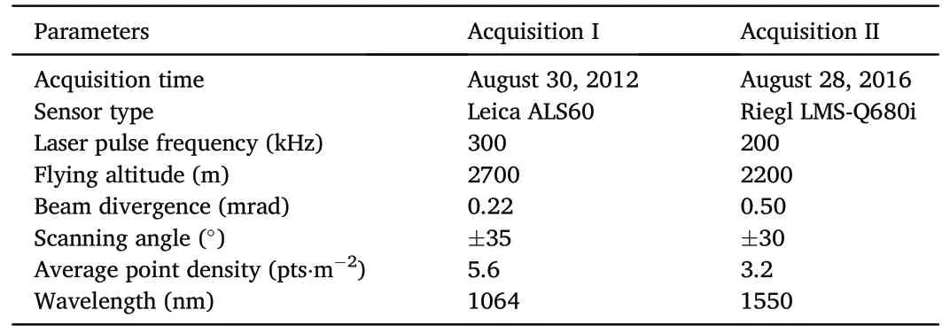
Table 1Characteristics of two ALS data acquisitions.

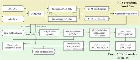
Fig.2.An overview of the workflow for estimating forest aboveground carbon dynamics using bi-temporal ALS data,including ALS data processing(i.e.,upper part)and aboveground carbon density (ACD) estimation (i.e., lower part) phases.

We preprocessed the raw LiDAR data into normalized point clouds and a canopy height model (CHM).We first used a cloth algorithm(Zhang et al.,2016)to classify the LiDAR point clouds of each survey into ground and non-ground points.In 2012, a DTM was created using the ground points with a grid size of 1 m.Next,the LiDAR point clouds were normalized by subtracting the height of the DTM from that of the 2012 point clouds.The 2012 DTM was used because the 2012 point cloud data had a higher average point density.To obtain a smoother CHM raster,the normalized point clouds were rasterized into CHMs at a 1-m resolution using the point to raster (p2r) interpolation algorithm (Khosravipour et al.,2014).All processing of the LiDAR point cloud data was performed using the lidR package(Roussel et al.,2020).

Many point-based metrics have been proposed in previous studies.However,in recent studies,some CHM-based metrics have been used as strong predictors of ACD (Asner et al., 2012).Point-based metrics can offer detailed insights into the spatial distribution of LiDAR returns.However,CHM-based metrics provide information on the canopy surface height at the scale of the CHM resolution.Herein,we computed not only point-,but also CHM-based metrics(Table 2).As the CHM resolution was 1 m, there were 900 pixels in each 30 m × 30 m field plot and pixels below 2 m were excluded.Considering the two-dimensional nature of the raster data,CHM-based metrics can only characterize the surface height information of the outer canopy.The CHM-based metrics used in this study mainly included: mean of canopy surface height (CHmean), standard deviation of canopy surface height (CHsd), coefficient of variation of canopy surface height (CHcv), canopy surface height percentiles(CH.p25, CH.p50, CH.p75,and CH.p95),and rumple index (RI).The RI was calculated as the ratio of the canopy surface area to the ground surface area(Jenness,2004).

We used only the first returns when computing point-based metrics because they are more closely related to changes in vegetation surface information,and points below 2 m were excluded.We computed various metrics related to the height,canopy volume,and structural complexity(Table 2).The height metrics included height statistics(e.g.,Hmean and Hske) and height percentiles (e.g., H.p25 and H.p50).Next, we used density metrics(e.g.,D.p20 and D.p50),canopy cover indices(CC,CCm,CRR,and CTHK),and canopy vertical profiles(LAD and LAI)to describe the vegetation canopy volume.Density metrics were calculated as the ratio of the points above the quantiles to the total number of points.The leaf area index(LAI)is defined as the area of leaves per unit ground area.The leaf area density(LAD)values are the partial volumetric components of LAI(Eq.(1)),which represents leaf area per height interval per canopy volume(de Almeida et al.,2019b).Some studies have demonstrated thatLAD and LAI are highly correlated with forest AGB(Bouvier et al.,2015;de Almeida et al., 2019a).Changes in the LAD vertical profile contain dynamic information regarding the horizontal and vertical canopy structures.The LAD function in the lidR package computes the LAD profile based on the method of Bouvier et al.(2015),which corrects the LiDAR point density for occlusion effects.We defined the height interval as 2 m and calculated 11 metrics[leaf area density above the height(e.g.,LAD6and LAD10), leaf area density between the height intervals (e.g.,LAD2_10and LAD10_20),and LAI].As a basic parameter for characterizing species diversity in biological systems, the Shannon vertical complexity index (SVCI) (Eq.(2)) measures canopy vertical structural diversity by quantifying distribution of point density or leaf area density across the profile (de Almeida et al., 2019a).Vertical complexity index (VCI) is a fixed normalized value of the SVCI.

Table 2Summary of the point- and CHM-based metrics using ALS data.

2.5.Feature selection and predictive modeling

The small number of field plots may have reduced the accuracy of the statistical models used to estimate forest parameters using LiDAR data.As there were only 20 revisited plots in 2016,we explored the 2012 ground data combined with area-based metrics to develop the ACD model and transfer this model to 2016 metrics.The temporal transferability of the model was assessed using revisited plot data.

Before predictive modeling, and while considering the existence of autocorrelation and multicollinearity among variables, the extracted metrics were filtered using the following steps:

(1) We performed correlation analysis on all 2012 metrics based on Pearson product-moment correlation coefficients (r) and deleted some metrics with r ＞0.8.(2) Based on the metrics selected in the previous step,a Wilcoxon matched pairs test with a confidence level of 0.05(p ＞0.05)was used to test whether there was a significant difference between each metric of the revisited plots in 2012 and 2016.Using independent variables with no significant differences can effectively improve the generality and transferability of the model(Navarro et al.,2020).

For modeling,we built multivariate linearity with the ACD from the 2012 field plots as the dependent variable and area-based metrics as the independent variables.To establish a linear relationship between the explanatory variables and their corresponding variables, a natural logarithmic transformation was applied to the subset of variables after filtering(Næsset et al.,2005).A multivariate linear model was chosen to model the ACD because other studies have shown that this method has better transferability than other machine learning methods(e.g.,random forests) when estimating forest parameters using ALS data (Zhao et al.,2018).A stepwise regression method based on bidirectional elimination was applied to select the feature variables used to establish the ACD prediction model.Bidirectional elimination is a combination of forward and backward eliminations.Each variable is added to the model through forward selection,and then the contribution of the variable is calculated according to the Akaike Information Criterion(AIC)(Akaike,1974),and finally the variable with a small contribution is removed by backward elimination.Three variables were used as the upper limit of the number of variables in the model,and the ordinary least squares method was used to estimate the optimal coefficients of the model.The multivariate stepwise regression process was implemented using the leaps package(Lumley and Miller,2004),which considers all possible combinations of variables and selects the optimal feature combination based on the adjusted R2.We used the model with the highest accuracy obtained in the aforementioned process as the prediction model for the 2012 ACD.The prediction accuracy of the model was evaluated via leave-one-out cross-validation (LOOCV) using the coefficient of determination (R2;Eq.(3)),root mean square error(RMSE,Eq.(4)),and relative root mean square error(rRMSE,Eq.(5)).The values of R2,RMSE,and rRMSE were calculated as follows:

2.6.Spatial extrapolation and ACD dynamic analysis

To estimate the wall-to-wall ACD distribution map across the study area, a series of 30 m × 30 m grids corresponding to the dimensions of the field plots were generated across the entire research area.Area-based metrics were derived for each 30 m ×30 m grid in 2012 and 2016 and the ACD of the two periods for each grid cell covering the study area was predicted based on the temporally transferable model.Based on a review of historical records and communication with local forestry practitioners,there were no significant disturbance events such as fires, storms, or insect outbreaks in the study area between 2012 and 2016.As a result,growth and mortality were assumed to be constant over a 4-year period.Subsequently, we calculated the absolute changes (Eq.(6)) and relative change rate of the ACD (Eq.(7)) between 2012 and 2016 using an indirect approach as follows:

where ΔACD and ΔACD% are the absolute and relative changes,respectively;ACDt2and ACDt1are the forest ACD estimates for the years t2and t1, respectively.ΔACD% has the advantage of being able to highlight regions where the absolute change in the ACD is low, but the growth rate may vary considerably.

Before analyzing the ACD changes, we classified the logging area at the 30-m grid-level according to the canopy height variation with reference to Dalponte et al.(2019).We excluded the effects of human interference because we wanted to focus more on the underlying patterns of ACD changes caused by natural factors.In the height change of the two-period CHM,if the height decrease was ＞50%of the canopy height in 2012,we classified this pixel as“logging”.At the 30-m grid-level,we classified the grid as “logging” if at least 20% of the pixels were in this class.The grid-level classification of logging areas based on the pixel level can effectively eliminate occasional situations in which the height of the canopy surface decreases owing to insufficient point density.

We investigated the relationships between ACD changes and dominant tree species, forest age group, topography, and canopy structural heterogeneity without human disturbance.Qualitative comparison and quantitative analysis of the spatial patterns of ACD changes were performed.In terms of the topographic data,we resampled the DTM to 30 m while keeping it aligned with the grid.The aspect was calculated using QGIS and divided into four categories: sunny slope (0-45°and 315°-360°), semi-sunny slope (45°-90°and 270°-315°), semi-shady slope (90°-135°and 225°-270°), and shady slope (135°-225°).The elevation was divided into three categories according to the elevation range in the study area: low (775-875 m), median (875-975 m), and high(975-1,079 m).Information on dominant tree species(larch,white birch, mixed, and other shrubs) and forest age groups (young, middleaged, near-mature, and mature) was obtained from the subcompartment data in 2012.

The Gini coefficient of the LiDAR height has been demonstrated to be a critical indicator for characterizing canopy structure attributes in boreal forest ecosystems(Valbuena et al.,2017)and has been used as an ancillary variable for ALS-based forest biomass estimation(Adnan et al.,2021).Considering the powerful capacity of the Gini coefficient to describe forest canopy structures at the stand level, we used it to quantitatively measure the heterogeneity of canopy surface height.The Gini coefficient ranges from 0 to 1, with a value of 0 indicating complete homogeneity and 1 indicating complete heterogeneity.We calculated the Gini coefficient for each 30-m grid according to an unbiased estimator developed by Glasser(1962):

where hiis the value of i-th 2012 CHM pixels inside the grid; hjis the value of j-th 2012 CHM pixels inside the grid;h is the mean value of 2012 CHM pixels inside the grid;n is the number of 2012 CHM pixels inside the grid.In this study, n is equal to 900, because there are 900 CHM pixels with a 1-m resolution in each 30 m grid.Fig.3 shows the CHMs and their overlay with the Gini coefficient for the three 300 m×300 m forest plots in the study area(Fig.1c).The overlay clearly demonstrates the different levels of canopy structure heterogeneity driven by the Gini coefficient in the three plots.

Finally,to understand whether the Gini coefficient could prove to be a useful indicator for characterizing ΔACD% in boreal forests, the Boruta algorithm (Kursa and Rudnicki, 2010) ranked the importance of all factors, where dominant tree species, forest age groups, aspect, and elevation were considered categorical variables, and the Gini coefficient was considered a continuous variable.The Boruta algorithm is built based on the random forest algorithm and evaluates the degree of importance of the explanatory variables to the corresponding variables according to the Z score (Kursa and Rudnicki, 2010).We also explored the quantitative relationship between the Gini coefficient and ΔACD%.The model was fitted,and its accuracy was evaluated using a 10-fold cross-validation.

3.Results

A total of 53 area-based metrics was calculated.After filtering using correlation analysis and the Wilcoxon matched-pairs test,23 point-based metrics(Hske,H.p10,H.p30,H.p50,H.p60,H.p70,H.p75,H.p80,D.p10,D.p40, D.p60, D.p80, D.p90, CC, CCm, LAD14, LAD18, LAD22, LAD26,LAD30, LAD10_20, LAD20_30, and SVCI) and three CHM-based metrics(CH.p50,CH.p95,and RI)were removed.The canopy height percentiles for upper height(i.e.,H.p95,H.p90),canopy vertical profile metrics(i.e.,LAD6,LAI),and mean canopy surface height(CHmean)were most often selected by multiple regression models(Fig.4).This suggests that these variables play an integral role in constructing the ACD model.Notably,none of the models selected density metrics to estimate ACD.Finally,we selected the best three-variable model as the prediction model for the ACD in 2012.The model formula was:

The LOOCV results showed that the model achieved high accuracy in estimating ACD, with R2and rRMSE of 0.91 and 17.21%, respectively(Fig.5a).Fig.6 shows a visual inspection of the results of the Pearson correlation analysis and Wilcoxon matched-pairs test conducted for the three explanatory variables.The Pearson's correlation among the three variables was low (Fig.6a).Moreover, the distribution of the three explanatory variables exhibited similarity across the 20 revisited plots(Fig.6b, c, and d), which indicate that there were no statistically significant differences for each variable between the two acquisitions of data.The utilization of these sufficiently robust variables formed the foundation for the model's capability to achieve transferability.

Fig.3.Example of canopy height models and corresponding Gini coefficient results for three squared forest plots in 2012 with low(a1 and a2),medium(b1 and b2),and high (c1 and c2) canopy structural heterogeneity with a size of 300 m × 300 m.

Fig.4.The independent variable selection results for predicting 2012 forest ACD with one-, two-, and three-variable statistical models using the stepwise linear regression method.

To evaluate the temporal transferability of the 2012 predictive model,it was applied to the 2016 metrics and compared in terms of R2and rRMSE(Fig.5).The results of the LOOCV procedure(Table 3)show that the difference in prediction accuracy between the fitted model directly obtained from the 2016 revisited plots and the transferable model was small.The RMSE and rRMSE predicted by the transferable model were slightly higher than those predicted by the fitted model(ΔRMSE=0.28 Mg·ha-1, ΔrRMSE = 0.78%), but the R2values were the same for both(R2= 0.87).This small discrepancy illustrates that the 2012 model captured the temporal transferability of the LiDAR metrics.Therefore,we used the temporal transferability of the 2012 model to predict the ACD changes using an indirect approach over two acquisitions.Compared to the results of the ΔACD% model (R2= 0.85, rRMSE% = 25.83%), the single-date ACD model had higher accuracy.

A wall-to-wall map of carbon dynamics at a 30-m resolution across the entire study area was predicted as the difference between the 2016 and 2012 ACD using an indirect approach(Fig.7).The average ACD went from 33.77±16.59(SD=standard deviation)Mg·ha-1in 2012 to 39.16± 16.35 (SD) Mg·ha-1in 2016, representing an increase of 15.96%.Overall, the average ΔACD was 5.38 ± 2.81 (SD) Mg·ha-1(Fig.8) and the carbon sequestration rate was 1.35±0.70(SD)Mg·ha-1·year-1.

We identified areas of human interference through canopy height variation,where 29%of the grids were classified as“logging.”The forest canopy surface height decreased vertically within a 30 m×30 m grid,as shown by the point cloud probability density and side-lateral views(Fig.9a and b).Meanwhile, in the grids with normal growth, both the CHM values and the point cloud probability demonstrate an increase in forest height (Fig.9c and d).To explore the spatial patterns of carbon dynamics under undisturbed conditions, these “logging” grids were removed.The statistical relationships between different forest stands,environmental factors,and the mean values of ACD changes are shown in Fig.10.

For different age groups (Fig.10a), near-mature stands had the highest gain of ΔACD, whereas ΔACD% in middle-aged stands was the highest, followed by young stands and mature stands that had a significantly lower gain.The birch-dominated stands had the highest accumulation of ΔACD%(Fig.10b).The birch-dominated stands also had the highest gain of ΔACD, followed by larch and mixed stands.When considering different elevation classes (Fig.10c), we observed that forests at lower elevations had the lowest gain of ΔACD, but the ΔACD%decreased with increasing elevation, and forests at higher elevations showed a slower relative change rate.The difference between the aspect and the ΔACD was small(Fig.10d),and the ΔACD%of sunny slope forest was slightly larger than that of shady slope.

The Boruta feature selection algorithm's importance ranking of explanatory variables for ΔACD%showed that the Gini coefficient had a significant impact on the ΔACD%,and the significance was much larger than the remaining four factors [Gini coefficient (45%) ＞age groups(18%)＞elevation(8%)＞dominant tree(3%)＞aspect(2%)].The Gini coefficient values ranged from a minimum of 0.02 to a maximum of 0.79,with a mean of 0.28 across the study site.In particular,we observed that the ΔACD% showed an upward trend with the increase of the Gini coefficient(Fig.11).Assuming an exponential relationship between the two variables,the fitted model is shown in Fig.11.The results of the 10-fold cross-validation exhibited that the rRMSE of the model was 40.90%and the R2was 0.61.

4.Discussion

ALS has been proven to provide detailed spatial predictions of forest parameters and could be a powerful tool for regional dynamic real-time monitoring of forest resources (Xiao et al., 2019; Huertas et al., 2022;Tymiˊnska-Czabaˊnska et al.,2022).Most previous studies have focused on these topics.In this study, we proposed a design idea for a temporally transferable model and used it as a general model to predict the carbon dynamics of boreal forests in China.Furthermore, we also attempted to use forest stand factors and environmental properties to understand and explain the spatiotemporal variations in ACD, which require urgent attention.As forests have dual functions as a carbon sink and carbon source, understanding the spatial patterns of carbon dynamics would help improve forest management and formulate reasonable development plans.

An increasing number of studies are seeking transferable and universal LiDAR-based models (Fekety et al., 2014; Sumnall et al., 2016;Karjalainen et al., 2018).The accuracy of applying existing forest attribute models to new sites depends on the modeling approach,consistency of stand conditions, and similarity of area-based metrics (Tompalski et al., 2019).In our study, the ACD in 2016 was successfully predicted using the temporal transferability of the linear model from 2012,and the results of the LOOCV procedure showed only a very slight decrease in its accuracy (ΔRMSE = 0.28 Mg·ha-1, ΔrRMSE = 0.78%).The average point cloud density in 2012 was nearly twice that of 2016 due to the various sensors,flight patterns,and configuration parameters used in the LiDAR data collection.However,according to the results of the Wilcoxon matched-pairs test, we found no significant difference in the statistical distribution between the point- and CHM-based metrics in a temporally transferable model (Fig.5a, b, and c).These results are consistent with previous research by Zhao et al.(2018).They estimated the forest aboveground biomass using multitemporal LiDAR data at different point densities and found that differences in the properties of the point clouds themselves did not affect the explained variance and accuracy of the model.They attributed this advantage to the fact that the laser scans were sampled according to the probability distribution.

Fig.5.Comparison of ALS- and field-based forest ACD estimation results for 2012 (a) and 2016 (b), respectively.Based on the temporally transferable model, the forest ACD of 2016 (c) and their dynamic changes (d) were also obtained successfully.

The choice of variables is critical to the generality of the model(Navarro et al.,2020).Three-variables model is a balance between model interpretability and accuracy.Increasing the number of variables beyond three only leads to a small improvement in precision (three-variable model:adjust R2=0.91,eight-variable model:adjust R2=0.93).In this study, our temporally transferable model not only finds the most stable metrics,but also utilizes the model with the best accuracy for ACD estimation.On the one hand,from the perspective of the selection of model feature metrics, CHmean, upper percentiles of height (i.e., H.p90 and H.p95),and canopy vertical profiles were selected multiple times by the model.Similarly, Knapp et al.(2018) reported that CHmean at various pixel resolutions outperformed any other metric for forest carbon stock and biomass prediction.As shown in Fig.4, some height metrics (i.e.,CHmean, Hmean, H.p40, and H.p90) were the generally preferred indicators for univariate models, but using height metrics only was not a consistent predictor of ACD (adjusted R2= 0.68-0.76).The addition of the LAD profile,which is estimated from laser pulse penetration,enables the information provided in the vertical direction of the canopy to be characterized,and its complementation with canopy height metrics can improve the prediction accuracy of ACD.However, we used a linear model instead of a machine learning model because the temporal transferability of linear models is easier to interpret than that of machine learning models(Zhao et al., 2013).Machine learning models are black boxes (Liang, 2007), and the nature of overfitting makes them less capable to reveal plausible transferable relationships than linear models.In the same stand environment, the temporal transferability of linear models was successfully applied to predict forest parameters using new data-collection methods(Tompalski et al.,2019).Although our proposed modeling approach utilizing the stable metrics enhances the transferability of the temporally transportable model,it is important to further investigate the predictive capability of the model when applied to different areas.Exploring its performance in diverse settings will provide valuable insights into its generalizability and effectiveness.

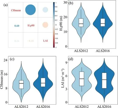
Fig.6.Three independent variables were inspected visually based on Pearson correlation analysis(r ＜0.8)and Wilcoxon matched-pairs test(p ＞0.05).The Pearson correlation coefficients between three optimum variables were calculated(a).Moreover,comparisons between the statistical distributions of the 90-percentile height(H.p90)(b),mean canopy height(CHmean)(c),and leaf area index(LAI)(d)independent variables for the forest ACD prediction model in 20 revisited plots using the violin plots.

Table 3Summary of ACD model performance and transferability assessment.

The quality and quantity of the samples had a non-negligible effect on the estimation of forest attributes(Gobakken et al.,2013;Fassnacht et al.,2014;Shin et al.,2016).Gobakken et al.(2013)reported that a stratified sample design contributed to producing fairly reliable predictions of forest structure attributes and that stratified models were more accurate than general models.Considering the impact of sample size and stratified sample design on forest attribute estimates, the 2012 field plots were more representative than the 2016 field plots.Our results showed that the 2016(R2=0.87,rRMSE=17.47%)model estimated the forest ACD directly using revisited field plots with lower precision than the 2012 model (R2= 0.91, rRMSE = 17.21%).This result is consistent with the findings of Liu et al.(2018).They suggested that 27-45 might be a suitable sample size range, with a smaller sample size increasing the sensitivity of LiDAR-based forest structural attribute estimates.As the 2016 samples were randomly selected for revisiting based on the 2012 samples,there was uncertainty,which may be one of the reasons for the decline in the accuracy of the 2016 ACD prediction model.

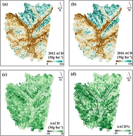
Fig.7.The spatially continuous maps of final forest ACD estimation results in 2012(a)and 2016(b)with a spatial resolution of 30 m for the whole study area.Insets c and d show the absolute(ΔACD)and relative change rates(ΔACD%)of forest ACD,with the carbon sink and carbon source areas represented by red and black colors,respectively.(For interpretation of the references to color in this figure legend, the reader is referred to the Web version of this article.)

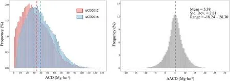
Fig.8.Histograms of ACD and ΔACD distributions for the entire study area.Dashed lines represent mean values.

Fig.9.Comparisons of canopy height models and corresponding vertical profiles of point cloud probability density for four forest plots with selective logging practices(a and b)and natural growth(c and d)in 2012 and 2016.The skylines of side-lateral views of each plot denoted as solid black lines show the decreasing or increasing trend of canopy heights in forest plots with a grid size of 30 m × 30 m.

Boreal forests play an important role in the global carbon cycle(Reich et al.,2014).Based on the literature,we know that Chinese boreal forests have been more productive in recent decades compared to those in Russia,Canada,and the United States(Jiang et al.,2002).In this study,the spatial prediction of ACD change demonstrated that forests in the entire study area were sequestering carbon at a rate of 1.35 Mg·ha-1·year-1, and the average ACD increased by 15.96%.Environmental differences may drive the various spatial patterns of carbon change.Therefore, we analyzed forest carbon dynamics under natural conditions from the perspectives of absolute and relative change rates.We focused more on the relative rate of change in ACD because absolute change reflects the accumulation of carbon, while the relative rate of change more strongly highlights the regrowth areas that are growing faster (Dalponte et al., 2019).In terms of age groups, we found that young and middle-aged forests accounted for a small proportion of the total ACD,but their growth rates were higher than those of near-mature and mature forests.Fu et al.(2021)performed a Lorey's mean height and volume change detection study in ginkgo-planted forest stands in China;their results showed that Lorey's mean height and volume increased significantly in middle-aged stands,and the growth rate was the lowest in mature stands.Our study was conducted in natural forests, and large differences in physiological and ecological characteristics between plantations and natural forests(Marcos et al.,2007;Cai et al.,2019)did not hinder the consistency of the results.Middle-aged stands play a critical role in carbon sequestration in forests.In particular, under the premise of little variation in the elevation range across the study area(775-1,079 m), we also observed an obvious trend in which ΔACD%gradually decreased with increasing elevation.Previous studies have indicated that forests on sunny or semi-sunny slopes tend to have a higher rate of ACD change than those on shady or semi-shady slopes(Dalponte et al.,2019).No such trend was observed in our study,which may have been caused by similar soil moisture and climatic conditions owing to the small height differences in the study area.Our study focused on a few key factors that affect carbon stocks.Remote sensing techniques have enabled researchers to retrieve environmental factors, such as light availability, disturbance intensity, and site quality, at the stand level(Coops et al.,2007;Chen and Zhu,2012;Goodbody et al.,2019;Fu et al.,2021).The next critical step is to explore these variables to underpin the study of LiDAR carbon dynamics.

In the present study, the Gini coefficient of the 2012 ALS-derived CHM described the heterogeneity of canopy surface heights at the stand level in a straightforward manner.This heterogeneity is manifested in two main aspects.First,as the individual trees within the stand grew,the canopies began to touch and shade each other.This is because of the competitive relationship between individual trees, which reflects the large inequality in canopy size(Forrester,2019).In addition,forest gaps affect the structure and composition of forests in both the horizontal and vertical directions.The diversity of the canopy structure affects factors such as light intensity and soil moisture, which influence forest growth(Stan and Daniels, 2014).The importance ranking of forest stands and environmental factors indicated that the Gini coefficient could be used as a single indicator to successfully explain most of the ΔACD%(R2=0.61,rRMSE=40.90%).Valbuena et al.(2017)found that the L-coefficient of variation (i.e., the Gini coefficient) and L-skewness calculated by the LiDAR height based on deductive mathematical rules describing distributions can be directly used to detect competition conditions in different forest areas and have great potential for describing natural regeneration in ecosystems.Canopy structure heterogeneity not only serves as an auxiliary variable in forest biomass modeling but also demonstrates its ability to reveal the forest carbon sequestration rate in our study.A growing body of research has demonstrated the potential of LiDAR in providing unambiguous quantitative spatial information on forest structural diversity (Mura et al., 2015; Martins-Neto et al., 2021).It is worth noting that the availability of light and its interception by the dominant canopy in boreal forests are the main factors limiting forest growth(Valbuena et al.,2017).In future,LiDAR data should be used to investigate and quantify the relationship between forest structure and carbon dynamics in various forest environments, including tropical and subtropical regions.

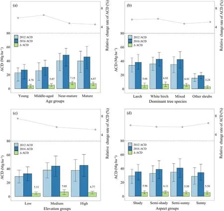
Fig.10.The bar graph depicts ACD and ΔACD within different forest stands and environment factors in 2012 and 2016.The line chart in the top of each bar graph corresponds to the ΔACD%.Classification according to the forest age groups (a), dominant tree species (b), elevation (c), and aspect (d).

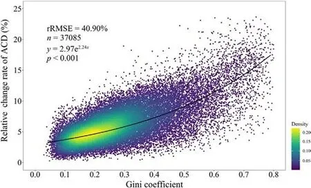
Fig.11.Scatter plot between ΔACD% values and Gini coefficients for all 30 m× 30 m grids in the whole study area and its corresponding exponential fitting model with statistical characteristics.

5.Conclusions

In this study, we used bi-temporal ALS data to estimate and map spatiotemporal variations of ACD over a 4-year period in the boreal natural forests in the GKM region.A method for temporally transferable model fitting was presented for modeling and estimating the absolute change and relative change rates of ACD.In addition, carbon dynamics were interpreted and analyzed based on dominant tree species, age groups, topography, and canopy structure heterogeneity for the whole study area.The results showed that the temporally transferable model including stable variables(R2=0.87,rRMSE=18.25%)was statistically equivalent to the model directly obtained by the 2016 revisited plots(R2=0.87,rRMSE=17.47%).Area-based approach ACD estimates showed that the average ACD gradually increased from 33.77 Mg·ha-1in 2012 to 39.16 Mg·ha-1in 2016 over the course of four years, an increase of 15.96%with a carbon sequestration rate of 1.35 Mg·ha-1·year-1.The Δ ACD%in middle-aged stands was the highest,followed by young stands,and significantly lower in mature stands.Further,we observed a greater rate of carbon accumulation at lower elevations.Overall, the Gini coefficient was the most important variable related to the ΔACD%across the entire study area.This study demonstrates the applicability of using bitemporal ALS data for mapping spatiotemporal variations of ACD and determining spatial patterns of carbon change, which are particularly valuable for carbon trading,REDD+and other goals aimed at achieving climate mitigation through forest management at all levels.

Funding

We acknowledge grants from the National Key R&D Program of China(Project Number: 2020YFE0200800) and National Science and Technology Major Project of China's High Resolution Earth Observation System(Project Number:21-Y20B01-9001-19/22-1).

Availability of data

Not applicable.

Authors’contributions

Zhiyong Qi and Shiming Li contributed equally to this work.Zhiyong Qi and Shiming Li: Conceptualization, Methodology, Formal analysis,Visualization,Investigation,Writing-original draft,Writing-review&editing.Yong Pang and Guang Zheng:Methodology,Writing-review&editing.Dan Kong: Methodology, Investigation.Zengyuan Li: Writing -review & editing, Funding acquisition, Project administration.All authors contributed to the finalization of the manuscript.

Declaration of competing interest

The authors declare that they have no known competing financial interests or personal relationships that could have appeared to influence the work reported in this paper.

Acknowledgments

The authors are grateful to the teachers and students who took part in the remote sensing campaigns and field data collection in study area,Genhe,Inner Mongolia,China.