Regularization by Multiple Dual Frames for Compressed Sensing Magnetic Resonance Imaging With Convergence Analysis

Baoshun Shi,,, and Kexun Liu

Abstract—Plug-and-play priors are popular for solving illposed imaging inverse problems.Recent efforts indicate that the convergence guarantee of the imaging algorithms using plug-andplay priors relies on the assumption of bounded denoisers.However, the bounded properties of existing plugged Gaussian denoisers have not been proven explicitly.To bridge this gap, we detail a novel provable bounded denoiser termed as BMDual,which combines a trainable denoiser using dual tight frames and the well-known block-matching and 3D filtering (BM3D)denoiser.We incorporate multiple dual frames utilized by BMDual into a novel regularization model induced by a solver.The proposed regularization model is utilized for compressed sensing magnetic resonance imaging (CSMRI).We theoretically show the bound of the BMDual denoiser, the bounded gradient of the CSMRI data-fidelity function, and further demonstrate that the proposed CSMRI algorithm converges.Experimental results also demonstrate that the proposed algorithm has a good convergence behavior, and show the effectiveness of the proposed algorithm.

I.INTRODUCTION

MAGNETIC resonance imaging (MRI) is a widely used medical imaging technique, but slow imaging speed limits its applications.Compressed sensing magnetic resonance imaging (CSMRI) [1] methods can address this issue by acquiring undersampledk-space data.But recovery of the original magnetic resonance (MR) images from undersampled measurements is an ill-posed problem [2], [3].To cope with this problem, priors are utilized to reduce solution space[4], [5].However, determining how to exploit priors for recovering high-quality images is a challenge.

To address the aforementioned issue, traditional modelbased algorithms use a regularization model that characterizes the inherent priors of the underlying image to formulate an imaging optimization problem, and solve it with proper solvers.Among existing regularization models, sparse regularization models that promote the sparsity of the underlying image in an image domain or a transform domain were preferred [6], [7].Another popular prior is non-local similarity.To exploit such priors, Quet al.[8] designed a patch-based nonlocal operator (PANO) to sparsify MR images.Moreover,the low-rank property of the similar image patches was explored in [9], and a smooth surrogate function was proposed.Jacobet al.[10] proposed a structured low-rank formulation, and provided a fast MRI algorithm by exploiting different continuous-domain signal priors.Different from the above ideas, Haldar and Setsompop [11] proposed the use of shiftinvariant linear prediction for MRI.The traditional modelbased CSMRI algorithms are interpretable, but the reconstruction quality still has room for improvement [7].In addition,the reconstruction speed of the traditional dictionary or tight frame learning methods is slow due to the time-consuming learning process [12].With the resurgence of artificial intelligence [13], deep neural networks (DNNs) were utilized to overcome the shortcomings of the traditional model-based CSMRI algorithms [14].Recent years have witnessed varieties of data-driven end-to-end DNNs [15].Hashimotoet al.[16] proposed an iterative reconstruction approach that utilizes U-Net andk-space correction to achieve better reconstructions compared to non-iterative DNNs.Deoraet al.[17]proposed a novel generative adversarial network (GAN) for CSMRI.They used a U-Net with dense and residual connections as the generator, and proposed a patch-based discriminator which combines structural similarity index-based loss.Other common DNNs are DAGAN [18] and RefineGAN [19].These DNNs can preserve details of the MR images with fast imaging speed, but their model architectures are uninterpretable [19], [20].Recently, model-based DNNs were proposed to alleviate this problem via unfolding iterative algorithms into DNNs [21].Yanget al.[22]-[24] combined the alternating direction method of multipliers (ADMM) and halfquadratic splitting (HQS) algorithms with data-driven DNNs,and achieved high-quality images.Schlemperet al.[25] proposed unfolded HQS to accelerate MR image reconstruction,while Wanget al.[26] proposed to train the same network with various loss functions in an unsupervised fashion.

Even if the interpretable shortcomings of DNNs can be overcome by the model-based DNNs, the lack of flexibility is still inevitable.The plug-and-play (PnP) imaging algorithms gradually become more popular due to their flexibility and empirically superior performance.Differing from the aforementioned model-based DNNs, the PnP imaging method exploits the priors via a Gaussian denoiser.Any effective Gaussian denoiser can be plugged into the PnP framework[27], but determining how to exploit the Gaussian denoiser is a challenge.Based on the manner of utilizing denoisers, existing PnP imaging algorithms can be classified into the following two classes.One is the PnP imaging algorithm based on the modular structure of the solver, and the other one is the imaging algorithm based on PnP regularization models.Specifically, for the former class, the proximal operator in the algorithm iterations solves a prior sub-problem that can be regarded as a denoising sub-problem.Therefore, a Gaussian denoiser is used to replace the proximal operator in its iterations.In fact, the seminal work [28] of PnP imaging approaches belongs to this class.The modular structure of the ADMM solver is considered by Venkatakrishnanet al.[28],and they replaced the proximal operator in ADMM with a Gaussian denoiser.Subsequently, this replacement is extended to other solvers [27], [29], [30].Empirically, replacing the proximal operator of a solver with a Gaussian denoiser is effective, but it is limited to solvers whose iterations contain proximal operators.An alternative is the PnP regularization strategy, the second class, which aims to design a regularization model using Gaussian denoisers.For this strategy, the key concern is determining how to model the relation between the underlying image and its filtered version by a Gaussian denoiser.The regularization by denoising (RED) [31] models this relation in the spatial domain, while the deep prior-based sparse representation regularization model [32] characterizes this relation in the transform domain.

The proper Gaussian denoiser in the PnP imaging algorithm is important for achieving high-quality images and analyzing convergence.Recently, the block-matching and 3D filtering(BM3D) denoiser [33] and the denoisers based on deep learning (deep denoiser) [34], [35] are preferable.In fact, when the PnP imaging strategy is utilized with CSMRI, the BM3D denoiser can work well, such as with the decoupled CSMRI framework [36] and denoising approximate message passing(D-AMP) [37].Moreover, the PnP algorithms with deep denoisers have achieved remarkable reconstruction quality[29], and some studies were devoted to analyzing the conditions on the deep denoiser, which can help PnP algorithms establish convergence.Ryuet al.[38] proposed a real spectral normalization method to train deep denoisers.By doing so,the Lipschitz condition is imposed on denoisers.Using such a deep denoiser, they theoretically proved the convergence of the plug-and-play forward-backward splitting (PnP-FBS) and plug-and-play ADMM algorithms.Similarly, Bohraet al.[39]proposed 1-Lipschitz deep spline networks which exploit the slope normalization to constrain the Lipschitz constant of the activation functions, and established the convergence analysis of the PnP algorithms with such averaged deonisers.Moreover, Teodoroet al.[40] provided convergence analysis of the PnP algorithms with the assumption that the denoiser is nonexpansive.Based on the fact that the denoiser can be expressed as a proximal map with respect to some regularizers, Gavaskar and Chaudhury [41] proved the fixed-point convergence of the ISTA framework (PnP-ISTA) using generic kernel denoisers.Different from these ideas of imposing constraints on the denoisers, Buzzardet al.[42] provided an interpretation of fixed points from the consensus equilibrium perspective.

Another constraint on the plugged denoiser is the bounded constraint.Chanet al.[43] analyzed the convergence with a bounded denoiser assumption.Subsequently, based on this assumption, many impressive plug-and-play imaging algorithms with convergence guarantee were developed [44].Inspired by [43], we attempt to prove the convergence of the CSMRI algorithm under the condition of diminishing noise levels and the assumption of bounded denoisers.A denoiser with the bounded property in the PnP imaging algorithm is beneficial for convergence analysis.However, there is not a provable trainable denoiser with bounded property.Most of deep denoisers are difficult to be proven as bounded denoisers due to some tricks of deep learning, such as residual learning and batch normalization.In this paper, we propose a trainable bounded denoiser using dual tight frames whose deep network architecture is interpretable, and the corresponding denoiser can be explicitly proved as a bounded denoiser.

As mentioned above, the PnP CSMRI algorithms can be divided into two classes.Do these two classes of algorithms have relationship? In this paper, based on a simple induction,we show that under the HQS solver [45], these two strategies are the same.Based on this observation, we propose a regularization model based on multiple dual frames.We develop an algorithm for the CSMRI problem formulations by using the proposed regularization model, and theoretically analyze the convergence of the proposed algorithm.Our main contributions are as follows:

1) We propose a trainable bounded Gaussian denoiser.Differing from traditional data-driven tight frames methods,which learn tight frames via alternating optimization, we exploit dual tight frames to elaborate a trainable denoiser that can be learned in a supervised learning manner.A deep thresholding network (DTN) built by a residual dense block(RDB) and a squeeze-and-excitation (SE) block is elaborated on to determine the thresholds from the input instances.By doing so, the thresholds that shrink the coefficients of the underlying image over the analysis tight frame are spatialvariant.To exploit complementary priors, we combine the trainable denoiser with the BM3D denoiser.

2) We propose a novel regularization model using multiple dual frames for CSMRI.A plug-and-play regularization model is derived via the HQS solver.We term this regularization model plugged by the BM3D frames and the trainable dual tight frames as ReBMDual.Since multiple dual frames are utilized, the ReBMDual model can deliver complementary priors, such as deep priors, non-local similarity, and sparsity.We apply the ReBMDual model into the CSMRI field, and experimental results demonstrate that the proposed CSMRI algorithm can achieve better reconstructions than benchmark CSMRI algorithms at various sampling ratios.

3) We demonstrate the convergence of the proposed CSMRI algorithm under a mild condition.On the theoretical side, we demonstrate that the proposed trainable denoiser, BM3D, and the combined denoiser are all bounded.To the best of our knowledge, this is the first time that the bounds of the trainable and BM3D denoisers are proven explicitly.Under the condition of diminishing noise levels, we prove that the proposed CSMRI algorithm converges based on the bounded property of the combined denoiser and the bounded gradient of the CSMRI data-fidelity function.Moreover, we verify the good convergence behavior of the proposed algorithm empirically.

The structure of this paper is as follows.To begin with, Section II presents existing PnP imaging methods.Section III introduces the proposed trainable denoiser, the combined denoiser, and the proposed ReBMDual model in details.The bound of the combined denoiser is also presented in this section.Section IV introduces the proposed CSMRI algorithm using the ReBMDual model, and shows the convergence analysis of the proposed algorithm.We present experimental simulations in Section V, and give a discussion of the convergence analysis in Section VI.Finally, concluding remarks and directions for future research are presented in Section VII.

II.EXISTING PLUG-AND-PLAY IMAGING METHODS

Based on the maximum a posteriori (MAP) criterion and the Bayes theorem, the imaging optimization problem using a regularization model can be formulated as

wherex∈RNorx∈CNrepresents the underlying image, andy∈CMrepresents the measurement.The first term in (1) is called the data-fidelity term which promotes the consistency of the reconstructed image with the measurements.The second termR(x) is the regularization term that enforces some desirable properties onto the unknown image.The trade-off of these two terms is controlled by the regularization parameter λ.In (1), Φ(·) represents the sampling operator.For different imaging applications, the sampling operators are different.

The imaging algorithms using traditional regularization models often exploit the priors explicitly.Alternatively, the PnP imaging methods exploit the priors implicitly.The seminal work is the so-called PnP ADMM algorithm [28], which iterates as follows (for thetth iteration):

where ρ is the penalty parameter,uis the scaled dual variable,andzis the auxiliary variable.Equation (2) can be solved by using the gradient descent solvers if the sampling operator is differentiable.In the PnP ADMM algorithm, (3) is solved by a Gaussian denoiserD(x(t)+u(t-1);σ).Here,x(t)+u(t-1)can be regarded as a noisy image, and σ represents the input noise standard deviation.The PnP ADMM algorithm delivers an idea that the proximal problem defined in (3) can be solved by a Gaussian denoiser approximately [43], [44].Based on this idea, the proximal operators in the fast iterative shrinkagethresholding algorithm, primal-dual algorithm, and projected gradient solvers were replaced by Gaussian denoisers [27].

More recently, differing from the spirits of the PnP imaging algorithms based on the solver structure, PnP regularization models were proposed.The RED model [31] assumes that the underlying image is uncorrelated with the filtered residual,i.e.,

whereRED(x) represents the RED model.The optimization problem using this regularization can be solved by the fixedpoint updating solver or the steepest-descent solver.Theoretically, the RED model can be utilized for CSMRI.

III.THE PROPOSED REBMDUAL REGULARIZATION MODEL

A. The Regularization Model Induced by HQS

In this work, we solve the problem defined in (1) by using the HQS solver.Given the auxiliary variablez, (1) can be recast as

To solve the above problem, the HQS solver iterates as follows:

and

Equation (7) that contains the forward imaging model can be regarded as an inversion step, while (8) can be regarded as a filter or denoising step.If we define[43], it is not difficult to show that (8) equals to

According to the idea of the PnP ADMM algorithm, (9) can be solved by an effective Gaussian denoiser, i.e.,

In summary, the problem defined in (6) can be solved via iterating the inversion and filter steps alternatively.Because of the heuristic nature of this method, we call this method as PnP HQS.This PnP HQS framework is designed based on the structure of the HQS solver.Therefore, the PnP HQS method belongs to the first class of PnP imaging methods.Moreover,

z(t-1)=D(x(t-1);σ)based on (10), we have.Substituting this equation into (7), we can recast (7) as

From (11), the regularization model can be written as (for thetth iteration)

Since the denoiser in (12) is flexible, the above regularization model is PnP.From the above simple deduction, we induce a PnP regularization model via the HQS solver.Under the HQS solver, the first class of PnP imaging methods equals the second one.The regularization model has the following advantages.

1)Smooth: The regularization model contains a simple quadratic term, and it is smooth at thetth iteration.

2)Effective: The regularization model using plug-and-play priors is beneficial for high-quality imaging.

3)Flexible: The regularization model can be easily utilized for solving other imaging inverse problems, and can be combined with advanced solvers, without limits in the solvers containing proximal operators.

B. The Proposed Trainable Denoiser Based on Dual Tight Frames

Under the condition of diminishing noise levels [46], the bounded property of the Gaussian denoiser plays an important role in the convergence guarantee of PnP imaging algorithms [29], [43].However, it is difficult to prove the bound of the deep denoiser due to its complicated network architecture.In this paper, we attempt to address this problem and propose a trainable denoiser whose bound can be proven explicitly.

1)Loss Function: Tight frames are effective frames for sparse representation models, and have been widely used in imaging algorithms.Compared with fixed tight frames, datadriven tight frames are preferable due to their adaptive ability.However, existing data-driven tight frames algorithms optimize the tight frame and frame coefficients alternately [12],which is time-consuming.Differing from this, we propose a tight frame network that can be trained in an end-to-end supervised learning manner.Moreover, to improve the representation ability of the single tight frame, we extend the single tight frame to dual frame networks.Formally, the denoiser using dual tight frames can be described as

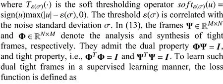
where λ1,λ2, and λ3are positive penalty parameters.

2)Deep Thresholding Network: The threshold in (13) is crucial to the performance of the denoiser.It can be set manually or updated by using the gradient descent optimizer.However,these methods ignore the spatial correlation of the image pixels.Based on this fact and the so-called universal threshold theorem proposed in [47], the thresholds should be different for each frame coefficient and related with the noise standard deviation σ [48], i.e., εi=ci·σ.Here εiis the threshold for shrinking thei-th channel of feature map, andciis the corresponding proportional constant.

Differing from the spirit in [48], which exploits the back propagation (BP) algorithm to learn the proportional constants, we propose the so-called CNet to determine these proportional constants from the input image.By doing so, the thresholds are instance-optimal and spatial-variant.Concretely, the adaptive thresholds can be written as

where ⊙ denotes the element-wise product, andmis the noise level map obtained by stretching the noise standard deviation σ.The size ofmis the same as that of learned proportional constant vectorc.To avoid arbitrary values, the elements ofcare limited to [cmin,cmax].Moreover, to extract the constants effectively, we use a RDB block [49] and a SE block [50] for CNet.We term the DNN determining the adaptive thresholds as DTN.Fig.1(a) shows the architecture of the proposed trainable denoiser termed as DualTF, wherein the DTN is jointly trained with dual tight frames in the training phase of the DualTF.

Fig.1.Illustration of the proposed DualTF denoiser and the proposed CSMRI-ReBMDual framework.(a) The architectures of the DualTF denoiser,DTN, and CNet.CNet contains a residual dense block and a SE block.In the SE block, the GAP represents the global average pooling layer, and FC represents fully connected layer; (b) The data flow graph of the proposed CSMRIReBMDual algorithm.

3)Bounded Property: Proving the bounded property of the proposed trainable denoiser explicitly is one of our main contributions, and Lemma 1 claims that the trainable denoiser is a bounded denoiser.

Lemma 1: Bound of the trainable denoiser: For any inputx∈RNand some universal constantL=(Here,cmaxdenotes the maximum element of proportional constant vectorc) independent ofM, the proposed trainable denoiser based on dual tight frames is bounded such that

Here,Mdenotes the dimension of the threshold vectore.

Proof: We assume that the analysis and synthesis of tight frames learned by the supervised learning method are strictly dual.In the experiment, these two frames may not be strictly dual.Under this scenario, we also present the convergence analysis of the proposed algorithm, and the detailed discussion can be found in Section VI.In this section, we assume that the learned frames Ψ ∈RM×Nand Φ ∈RN×Msatisfy the dual constraint strictly.Therefore, we have

Equation (18) can be recast as

Here, we usee∈RMto represent the threshold vector whose elements are utilized for shrinking Ψx.Let (Ψx)irepresents thei-th element of Ψxand εidenotes thei-th element ofe.The soft thresholding operatorT[(Ψx)i,εi] is defined as

We consider the shrinking processT(Ψx,e), one of the following situations will happen.

C1: Any element of Ψxsatisfies ( Ψx)i<-εi, thenT(Ψx,e)=Ψx+e.Therefore,

C2: Any element of Ψxsatisfies | (Ψx)i|≤εi, thenT(Ψx,e)=0.Therefore,

C3: Any element of Ψxsatisfies ( Ψx)i>εi, thenT(Ψx,e)=Ψx-e.Therefore,

C4: Any two or all three of the above situations may occur.C4 is a union of C1, C2, and C3.Therefore, as long as we find the upper bound of ||Ψx-T(Ψx,e)|under the C1-C3, the upper bound of that under C4 will be determined.Hence,when C4 occurs, the upper bound of ||Ψx-T(Ψx,e)is the maximum upper bound of the first three situations.Based on(21)-(23), we have

Recall the definition of threshold vectore=c⊙m, and each element of the proportional constant vectorschas a limited rangeci∈[cmin,cmax].Let εmax=cmax·σ denote the maximum element ofe.Thus

According to (19), (24), and (25), we can get

C. BM3D Denoiser and Its Bounded Property

The learned dual tight frames can capture the characteristics of the training dataset, but ignore the internal priors of the input testing images, such as non-local similarity.To alleviate this problem, we combine the well-known BM3D denoiser with the proposed trainable denoiser.In this section, we first introduce the frame representation of the BM3D denoiser which has been applied to image deblurring [51], and then exploit the frames to remove noise.Finally, we demonstrate the bounded property of the BM3D denoiser which is important for convergence analysis.

1)Frame Representation of the BM3D Denoiser: Firstly, we introduce the matrix [33] and frame representations [51] of analysis and synthesis BM3D operations.Letxn∈RNbe a noisy image, andRixn∈Rnbe theith image patch extracted from the noisy imagexn.Here, matrixRi∈Rn×Nrepresents the operator that extracts the patch from the whole image.The total number of image patches in each group is a fixed numberK, and the total number of groups isR.LetJr={ir,1,...,ir,k}be the set of image patch indexes in therth group, thus grouping can be defined byJ={Jr:r=1,...,R}.Based on these notations, the explicit matrix representation of the BM3D analysis operation can be written as

wherewrepresents the joint 3D groupwise spectrum, and ΨBM3DRis defined as

where ⊗ represents the Kronecker matrix product.The 3D decorrelating transform is constructed as a separable combination of 2D intrablock and 1D interblock transforms.Here,each block is an image patch.In (28),diis theith column of 1D interblock transformD1, andD2represents the 1D transform that constitutes the separable 2D intrablock transform.

The synthesis matrix is derived similarly.The estimated image is the weighted mean of the groupwize estimation, and the weights are defined asgr>0.The synthesis representation model for a noisy image can be represented as

D. The Proposed ReBMDual Model Using Multiple Dual Frames

According to (13) and (33), the combined denoiser can be formulated as

wherekis a trade-off factor of the two denoisers.The combined denoiser termed as BMDual can fuse deep priors and non-local similarity for high-quality imaging.In the following, we demonstrate the bounded property of the BMDual denoiser and introduce the proposed ReBMDual model utilizing the BMDual denoiser.

Based on Lemmas 1 and 2, Theorem 1 claims the bounded property of the BMDual denoiser.

Theorem 1: Bound of the BMDual denoiser.For any inputx∈RN, the BMDual denoiser based on Lemmas 1 and 2 is bounded such that

Proof: Based on (16) and (34), we have

Substituting (43) into the PnP regularization model (12), we can rewrite (12) as

Equation (45) is the so-called ReBMDual regularization model.

IV.THE PROPOSED REBMDUAL MODEL FOR CSMRI

A. Problem Formulation

In this section, we exploit the ReBMDual model to address the CSMRI problem.In the CSMRI field, the measurements are the partial Fourier transform coefficients.Mathematically,the sampling model of CSMRI can be described as

wherex∈RNorx∈CNis the underlying MR image,n∈CMis the Gaussian noise,Fu∈CM×Nrepresents the partial Fourier transform, andy∈CMis the measurement vector.The sampling ratio is defined asratio=M/N.Under the low sampling ratios, recovering high-quality images from the undersampled measurements is a challenge.We attempt to address this issue by using the ReBMDual model.According to (11), a CSMRI formulation can be described as (for thetth iteration)

In (47), the first term is the data-fidelity term, the second term is ReBMDual regularization model, and β is a trade-off parameter.

B. The Proposed CSMRI Algorithm

1)Inversion Step: Note that the objective function of formulation (47) contains two simple quadratic terms with respect tox, we can obtain its closed-form solution by zeroing the derivative of its objective function.The closed-form solutionx(t)should satisfy

whereHrepresents the conjugate transpose.The Fourier transformFis an unitary matrix admittingFHF=I, thus, the above equation can be rewritten as

which can be rewritten as

whereS0=andS(t)=FDBMDual(x(t-1);σ).Once the updated coefficients inkspace are at hand, the recovered image can be obtained via the inverse Fourier transform ofFx(t).Since the ReBMDual model is utilized for CSMRI, we term this algorithm as CSMRI-ReBMDual.To explain the CSMRI-ReBMDual algorithm clearly, a detailed description of our algorithm is presented in Algorithm 1, and the data flow graph is showed in Fig.1(b).Specifically, one iteration of the CSMRI-ReBMDual algorithm contains two modules,i.e., the denoising and inversion modules.In the denoising module, the BM3D and the DualTF denoisers are utilized.

2)Parameter Setting: We exploit the adaptive update rule instead of choosing a constant β.The adaptive update rule considers the relative residue

C. Convergence Analysis of the CSMRI-ReBMDual Algorithm

Due to the inversion and filter steps in the PnP imaging algorithms, the convergence analysis of these algorithms is difficult.We attempt to address this challenge in this section.In previous sections, we have given the bound of the BMDual denoiser.Based on this bound, we will show the convergence analysis of the proposed CSMRI-ReBMDual algorithm.Before we show the full proof, we first present a lemma,which is important for convergence analysis.Lemma 3 indicates that the gradient of the CSMRI data-fidelity function is bounded.The proof of Lemma 3 is based on the special structure of the CSMRI sampling matrix, and the detailed proof can be found as follows.

thus, we have

Since ||Fux||2≤||Fx||2=||x||2and the pixel values in the imagexare normalized into [0,1], we obtain

In (54), ||y||2=||Fuxori+n||2and ||n||2≤κ; here,xoriis the original image whose pixel values are normalized into [0, 1].Therefore,

Substituting (55) and (56) into (54), we get

Based on Theorem 1 and Lemma 3, Theorem 2 establishes the convergence of the proposed CSMRI-ReBMDual algorithm.

Theorem 2: Stable convergence of the CSMRI-ReBMDual algorithm.Consider the CSMRI sampling modely=Fux+n.Given{y,Fu},xissolved iteratively viatheCSMRI-ReBMDual algorithm, thenx(t)will converge.Thatis, there existsx∗such that | |x(t)-x∗||2→0 ast→+∞.

Proof: Let Θ be the domain ofx(t)for allt.On the domain Θ, we define a distance functiond: Θ ×Θ →R such that

We consider the aforementioned adaptive updating rule of the parameterβ.If Case 1 holds, then using Lemma 4 of Appendix A,x(t)satisfies

If Case 2 holds, according to the condition∆(t)<η∆(t-1), we have

As the iteration increases, i.e.,t→∞, one of the following cases must hold:

S1: Case 1 happens for infinitely manyt, but Case 2 happens for finitely manyt.

S2:Case 2 happens for infinitely manyt, but Case 1 happens for finitely manyt.

S3: In the early finite iterations, Case 1 or Case 2 occurs for finitely manyt, and then, both Case 1 and Case 2 occur for infinitely manyt.

S4: Both Case 1 and Case 2 occur for infinitely manytoften.

Convergence is established for S1, S2, S3, and S4 as follows.

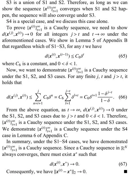
When S1 happens, there must exist aT1such that fort≥T1only Case 1 holds.Thus, using Lemma 4, fort≥T1, we can conclude that

whereC3is a constant.

When S2 happens, there must exist aT2such that fort≥T2only Case 2 holds.Thus, we have

V.EXPERIMENTS

A. Experimental Setup and Implementation Details

We randomly choose thirty T-1 weighted MR images of brain from the MICCAI 2013 grand challenge dataset [52] and thirty knee MR images from the MRNet dataset [53] with the coronal view as testing images.The size of each MR image is 256×256, and all the pixel values in these original images are in the range of [0, 1].Thek-space data is simulated by applying the 2D discrete Fourier transform to the original MR images.Two different types of sampling schemes, such as 1D Cartesian sampling and pseudo-radial sampling, are used to sample thek-space data.To simulate the practical sampling case, we add the Gaussian white noise with the standard deviation 0.1 onto the cleank-space data.Our simulations were performed on a computer with the NVIDIA GTX 2080Ti GPU using PyTorch.

1)Training Details of the Trainable Denoiser: The training and validation datasets of brain images including 4000 and 500 pieces are chosen randomly from the MICCAI 2013 grand challenge dataset, while the knee dataset with the same size of brain dataset is chosen randomly from the MRNet dataset.The totalnumber ofepochsis70,and the batchsizeis 8.Initially, weset thelearningrateas 1×10-3, and after 40 epochs, the learning rate decreases to 1×10-4.The hyper parameters of the loss function are set as λ1= λ2= 0.002, and λ3= 0.001.The number of learnable parameters in the proposed trainable denoiser is 1484 K.Moreover, the time to train the proposed bounded denoiser on a GTX 2080Ti is 12 hours, and the average time to denoise a noisy image with a size of 2 56×256 is 5.53 s.

B. Performance Verification of the Proposed Combined Denoiser

In order to show the effectiveness of the proposed combined denoiser, we compare the denoising performance of the BM3D [33], DnCNN [34], RDDCNN [56], MWDCNN [57],and BMDual denoisers.In the experiment, the trade-off factorkin the combined denoiser is set as 0.8.We retrain the blind models of the above mentioned deep denoisers, and we use the publicly available codes with the default parameter settings for the benchmark algorithms.The training, validation,and testing datasets including 4000, 500, and 30 pieces of knee images are chosen randomly from the MRNet dataset,and the size of each image is 256×256.Moreover, the noisy images are generated by adding Gaussian white noise with noise level σ ∈[0,75] to clean images.At different noise levels, the average peak signal-to-noise ratio (PSNR) values achieved by the various denoisers on thirty testing MR images are presented in Table I.From Table I, we can observe that the MWDCNN denoiser can obtain the highest PSNR values for all parts due to the advanced network architecture.Meanwhile, the BM3D denoiser, a traditional denoiser, obtains the lowest PSNR values.Among these algorithms, the results of the proposed combined denoiser are slightly lower than those of the MWDCNN denoiser.Nevertheless, the proposed combined denoiser can obtain better denoising results than those of the BM3D, DnCNN, and RDDCNN denoisers.Most importantly, our proposed combined denoiser is interpretable,and can be explicitly proved to be a bounded denoiser.To further improve the performance of our proposed denoiser, we can increase the network depth of CNet or apply transformer in CNet, and these are leaving for future research.

TABLE I THE PSNR VALUES ACHIEVED BY DIFFERENT DENOISERS AT NOISE LEVELS OF 15, 20, 25, 55, AND 75.WE REPORT THE AVERAGE PSNR VALUES (DB) ON THIRTY TESTING MR IMAGES.THE BEST TWO RESULTS ARE HIGHLIGHTED IN RED AND BLUE COLORS, RESPECTIVELY

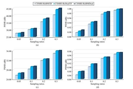
Fig.2.The average PSNR and SSIM results achieved by the CSMRI-ReBM3D, CSMRI-ReDualTF, and CSMRI-ReBMDual algorithms, respectively, under the 1D Cartesian sampling mode.The first row is the comparison of PSNR/SSIM vs.sampling ratios for brain MR images, and the second row is the comparison of PSNR/SSIM vs.sampling ratios for knee MR images.

C. The Power of the Combined Denoiser

To demonstrate the effectiveness of the BMDual denoiser,the plug-and-play CSMRI framework using a single denoiser is regarded as the benchmark algorithm.We use the peak signal-to-noise ratio (PSNR) and structure similarity index measure (SSIM) values to evaluate the reconstruction quality.The PSNR value between imagesxandxˆ is calculated as

whereMAXiis the maximum possible value of the image pixels andMS Edenotes the mean squared error.The SSIM value between imagesxandxˆ is calculated as

where σxxˆis the covariance ofxandµi, σiis the mean and variance of samplei, and the parametersc1,c2are smooth parameters.

Figs.2 and 3 report the average PSNR and SSIM values achieved by three different CSMRI algorithms named CSMRIReBM3D, CSMRI-ReDualTF, and CSMRI-ReBMDual at the sampling ratios of 0.05, 0.1, 0.2, and 0.3 via 1D Cartesian sampling and pseudo-radial sampling, respectively.At each sampling ratio, the average PSNR and SSIM values are the mean values of the thirty testing MR images.We can observe that the CSMRI-ReDualTF algorithm can achieve higher PSNR and SSIM values than those of the CSMRI-ReBM3D algorithm at the most cases and the CSMRI-ReBMDual algorithm using the combined denoiser can achieve the highest PSNR and SSIM values at various sampling ratios.Since the CSMRI-ReBMDual algorithm can exploit multiple complementary priors, it outperforms the ones using single denoiser in terms of the PSNR and SSIM values.

Fig.3.The average PSNR and SSIM results achieved by the CSMRI-ReBM3D, CSMRI-ReDualTF, and CSMRI-ReBMDual algorithms, respectively, under the pseudo-radial sampling mode.The first row is the comparison of PSNR/SSIM vs.sampling ratios for brain MR images, and the second row is the comparison of PSNR/SSIM vs.sampling ratios for knee MR images.

D. Comparison With Previous CSMRI Algorithms

To demonstrate the effectiveness of the proposed CSMRIReBMDual algorithm, we compared the performance of the proposed algorithm with the existing CSMRI algorithms including DLMRI [7], NLR [9], PANO [8], BM3D-MRI [36],BM3D-AMP [37], and RealSN-ADMM [38] at various sampling ratios.For fair comparison, we tuned the parameters that perform optimally for the aforementioned algorithms based on the maximum PSNR principle, i.e., fixing other parameters,tuning one parameter finely until obtaining the maximum PSNR.Moreover, we used the same initial guess for all the CSMRI algorithms, i.e., the zero-filled image.Table II presents the average PSNR (dB) and SSIM values achieved by the CSMRI algorithms at the sampling ratios of 0.05, 0.1, 0.2,and 0.3.The best results are highlighted in bold.For most parts, we can observe from the table that the PSNR values of the DLMRI algorithm are the worst.In terms of the PSNR and SSIM values, the NLR, PANO, and BM3D-based algorithms are better than the DLMRI algorithm.Moreover, the reconstructions of RealSN-ADMM are better than those of other benchmark algorithms owing to the advanced denoiser.Among these algorithms, the CSMRI-ReBMDual algorithm can achieve the highest PSNR/SSIM values for all parts due to the utilization of multiple dual frames.For example, in the case of the pseudo-radial sampling for the brain dataset, the average PSNR value of the CSMRI-ReBMDual algorithm can increase by nearly 5.69 dB, 3.9 dB, 3.8 dB, 3.45 dB, 1.68 dB,and 1.69 dB, compared to those achieved by the DLMRI,NLR, PANO, BM3D-MRI, BM3D-AMP, and RealSNADMM algorithms, respectively.In the case of the Cartesian sampling for the knee dataset, the average PSNR value of the CSMRI-ReBMDual algorithm can increase by nearly 1.98 dB,1.43 dB, 1.64 dB, 1.15 dB, 1.47 dB, and 0.52 dB than those achieved by the DLMRI, NLR, PANO, BM3D-MRI, BM3DAMP, and RealSN-ADMM algorithms, respectively.

To further evaluate the CSMRI algorithms, we present some reconstructions achieved by these algorithms in Figs.4-6.From the figures, we can observe that the reconstructions achieved by the DLMRI algorithm lose a large amount of detail information.The NLR, PANO, and BM3D-based algorithms can suppress some artifacts, but those reconstructions contain significant noise.The reconstructions achieved by the RealSN-ADMM are better than those obtained by the aforementioned algorithms.Moreover, the proposed CSMRI-ReBMDual algorithm can not only preserve most details but also reduce the noise.The proposed CSMRI-ReBMDual algorithm can achieve the best reconstructions among the seven algorithms in terms of visual quality.

E. Practical Convergence Behaviors

Earlier, we demonstrated the convergence of the proposed CSMRI-ReBMDual algorithm theoretically.To further evaluate the convergence behavior of the proposed algorithm, we present the curves of PSNR and SSIM versus iterations at the sampling ratios of 0.05, 0.1, 0.2, and 0.3 under different datasets and sampling modes in Fig.7.With the growth of theiterations, the PSNR and SSIM values become stable ultimately.From the figures, we can observe that the algorithm converges to a stable point at nearly 300 iterations.This result indicates the good convergence behavior of the proposed CSMRI-ReBMDual algorithm.In other words, on the practical side, the CSMRI-ReBMDual algorithm is convergent,which is consistent with the theoretical analysis.

TABLE II PSNR (DB)/SSIM RESULTS ACHIEVED BY THE CSMRI ALGORITHMS AT VARIOUS SAMPLING RATIOS UNDER DIFFERENT DATASETS AND SAMPLING MODES.AVERAGE REFERS TO THE AVERAGE VALUE OF DIFFERENT SAMPLING RATIOS

VI.DISCUSSION

In this section, we discuss the convergence of the proposed CSMRI algorithm under the case of the approximately dual constraint.We optimize the loss function defined in (14) to make frames meet the dual property as much as possible.However, during the experiment, we cannot guarantee the resulting frames Ψ∗and Φ∗to be strictly dual.In other words,the learned frames may be approximately dual.One way to address this limitation is deriving an orthonormal matrix from Ψ∗or Φ∗, which can be obtained by the singular value decomposition.However, imposing a strict constraint on the learned frames limits the expressivity of the network and increases its complexity [58].Therefore, we select the nearest dual matrix in the Frobenius norm sense.In this section, we discuss the bounded property of the trainable denoiser under the case of approximately dual tight frames.

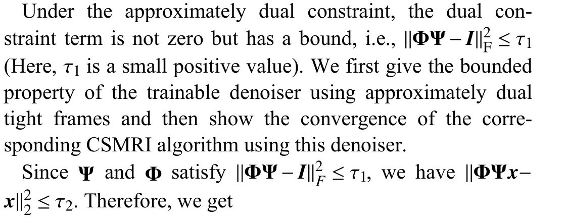
Fig.4.At the case of sampling ratio 0.1, the knee images recovered by the CSMRI algorithms under the Cartesian sampling mode.From left to right, and top to bottom: the original image (a), and the images recovered by (b) DLMRI (PSNR = 26.19 dB, SSIM = 0.7987); (c) NLR (PSNR = 27.07 dB, SSIM = 0.8208);(d) PANO (PSNR = 26.33 dB, SSIM = 0.8017); (e) BM3D-MRI (PSNR = 26.47 dB, SSIM = 0.8001); (f) BM3D-AMP (PSNR = 26.29 dB, SSIM = 0.7930);(g) RealSN-ADMM (PSNR = 28.04 dB, SSIM = 0.9022); (h) CSMRI-ReBMDual (PSNR = 29.01 dB, SSIM = 0.9145).The red arrow refers to the reconstruction of edge information.

Fig.5.At the case of sampling ratio 0.2, the knee images recovered by the CSMRI algorithms under the pseudo-radial sampling mode.From left to right, and top to bottom: the original image (a), and the images recovered by (b) DLMRI (PSNR = 31.42 dB, SSIM = 0.8673); (c) NLR (PSNR = 31.41 dB, SSIM =0.9056); (d) PANO (PSNR = 30.07 dB, SSIM = 0.8602); (e) BM3D-MRI (PSNR = 32.67 dB, SSIM = 0.9178); (f) BM3D-AMP (PSNR = 31.46 dB, SSIM = 0.9119);(g) RealSN-ADMM (PSNR = 33.12 dB, SSIM = 0.9597); (h) CSMRI-ReBMDual (PSNR = 33.70 dB, SSIM = 0.9642).The red arrow refers to the reconstruction of edge information.

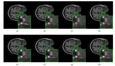
Fig.6.At the case of sampling ratio 0.2, the brain images recovered by the CSMRI algorithms under the Cartesian sampling mode.From left to right, and top to bottom: the original image (a), and the images recovered by (b) DLMRI (PSNR = 32.12 dB, SSIM = 0.8679); (c) NLR (PSNR = 32.07 dB, SSIM = 0.9216);(d) PANO (PSNR = 32.10 dB, SSIM = 0.8993); (e) BM3D-MRI (PSNR = 32.89 dB, SSIM = 0.9340); (f) BM3D-AMP (PSNR = 32.13 dB, SSIM = 0.9309);(g) RealSN-ADMM (PSNR = 34.07 dB, SSIM = 0.9712); (h) CSMRI-ReBMDual (PSNR = 35.19 dB, SSIM = 0.9773).The red arrow refers to the reconstruction of the white gap between the two black blocks.

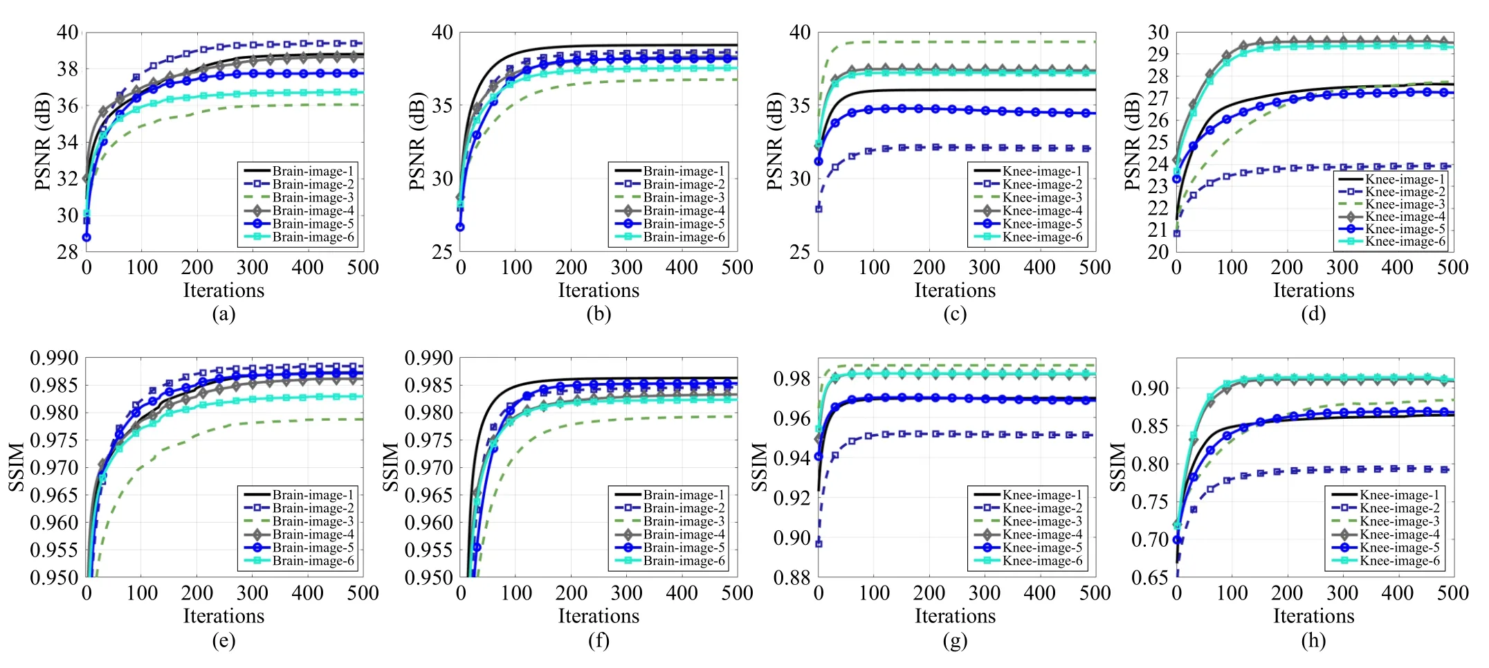
Fig.7.The first row shows the curves of PSNR versus iterations in the case where (a) the sampling ratio equals 0.2 with Cartesian sampling of brain images,(b) the sampling ratio equals 0.1 with the pseudo-radial sampling of brain images, (c) the sampling ratio equals 0.3 with the Cartesian sampling of knee images,and (d) the sampling ratio equals 0.05 with the pseudo-radial sampling of knee images, respectively.The second row shows the curves of corresponding SSIM versus iterations.

According to the proof in Lemma 1, similar results can be obtained

Inequality (71) indicates that the proposed trainable denoiser is bounded.Thus, the combined denoiser is bounded.Based on (44), we have

Under the approximately dual constraint, we can give the proof of convergence behavior based on the above bounded property of the combined denoiser.Concretely, we only need to modify some proofs in Lemma 4 as follows:

VII.CONCLUSION

In this paper, we proposed a trainable bounded denoiser,and combined it with the BM3D denoiser for building a combined denoiser.Moreover, based on the structure of the HQS solver and a combined denoiser, we proposed the so-called ReBMDual regularization model.The proposed ReBMDual model is flexible, which can act as an explicit regularization term for solving imaging inverse problems, not limited to the CSMRI problem.Based on the bounded gradient of the CSMRI data-fidelity function and the bounded property of the combined denoiser, we proved the convergence of the proposed CSMRI algorithm.Experimental results demonstrated that the proposed CSMRI algorithm could achieve better reconstructions than the benchmark CSMRI algorithms, and also confirmed the good convergence behavior of the proposed algorithm.

On the practical side, the proposed ReBMDual model has shown high imaging performance.Determining how to improve reconstruction quality is still a problem.One method to solve this issue is by exploiting the deep denoiser based on the transformer.Moreover, applying the trainable denoiser to multi-coil MRI will be a future research direction.

On the theoretical side, our work is the beginning of analyzing the plug-and-play CSMRI algorithm of utilizing a specific denoiser.The convergence of the proposed algorithm has been demonstrated, but determining how to design a plug-and-play CSMRI algorithm with the provable global convergence is still a challenge.Moreover, the theoretical analysis of the imaging method utilizing a deep denoiser is an open problem.We leave these for further study.

APPENDIX A PROOF OF LEMMA 4

Lemma 4: At thetth iteration, if Case 1 holds, then

for some constantsC3.

Proof: Let us consider the proposed formulation

Based on the first order optimality, we have

We assume that the optimal solution isx(t)at thetth iteration.Substituting this solution into the above equation yields

At thetth iteration, the value ofβfor updating image is β(t-1).Using the Lemma 3, we have

Based on this bound and Theorem 1, we obtain

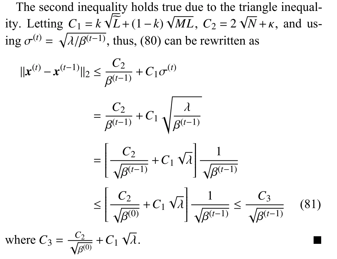
APPENDIX B PROOF OF LEMMA 5

Lemma 5: Regardless of S1-S3, for anyt, the sequencealways satisfies

for some constantsC6and 0 <δ<1.

Proof: For any case S1-S3, at thetth iteration, it holds that

APPENDIX C PROOF OF LEMMA 6

APPENDIX D PROOF OF LEMMA 7

Lemma 7: For the residuals ∆(t)=d(x(t),x(t-1)) under the S4 case, there exists a PGS {zt}t≥1such that ∆(t)≤ztfor allt.

Proof: The S4 case claims that both Case 1 and Case 2 occur for infinitely manyt, often.In other words, both Case 1 and Case 2 are visited infinitely often.Therefore, Case 1 may hold for finitely manyt, and then Case 2 holds for finitely manyt.Alternatively, Case 2 holds for finitely manyt, and then Case 1 holds for finitely manyt.We call the first time that both Case 1 and Case 2 occurs as the first round, and call the second time as the second round, and so on.Letn1be the iteration where Case 1 occurs for the first time, andm1>n1be the iteration where Case 2 occurs for the first time.Letn2>m1be the iteration where Case 1 occurs for the first time afterm2, andm2>n2be the iteration where Case 2 occurs for the first time aftern2.At the first round, Case 1 is visited for the iterationsn1,n1+1,...,m1-1 and Case 2 is visited for the iterationsm1,m1+1,...,n2-1.For each roundj≥1, Case 1 occurs at iterationst∈{nj,nj+1,...,mj-1} and Case 2 occurs at iterationst∈{mj,mj+1,...,nj+1-1}.To complete the proof, we should demonstrate that there exists a PGS {zt}t≥1such that ∆(t)≤zt.Now, we discuss this bound for Cases 1 and 2, respectively.

1)Case 1: For each roundj, Case 1 holds at iterationst∈{nj,nj+1,...,mj-1}, and based on the adaptive update role, we get

Using Lemma 4, we have