Modulation recognition network of multi-scale analysis with deep threshold noise elimination＊#

Xiang LI ,Yibing LI ,Chunrui TANG ,Yingsong LI

1College of Information and Communication Engineering, Harbin Engineering University, Harbin 150001, China

2Key Laboratory of Advanced Marine Communication and Information Technology, Ministry of Industry and Information Technology,Harbin Engineering University, Harbin 150001, China

3China Coal Technology Engineering Group Chongqing Research Institute, Chongqing 400037, China

4State Key Lab of Methane Disaster Monitoring &Emergency Technology, Chongqing 400039, China

Abstract: To improve the accuracy of modulated signal recognition in variable environments and reduce the impact of factors such as lack of prior knowledge on recognition results,researchers have gradually adopted deep learning techniques to replace traditional modulated signal processing techniques.To address the problem of low recognition accuracy of the modulated signal at low signal-to-noise ratios,we have designed a novel modulation recognition network of multi-scale analysis with deep threshold noise elimination to recognize the actually collected modulated signals under a symmetric cross-entropy function of label smoothing.The network consists of a denoising encoder with deep adaptive threshold learning and a decoder with multi-scale feature fusion.The two modules are skip-connected to work together to improve the robustness of the overall network.Experimental results show that this method has better recognition accuracy at low signal-to-noise ratios than previous methods.The network demonstrates a flexible self-learning capability for different noise thresholds and the effectiveness of the designed feature fusion module in multi-scale feature acquisition for various modulation types.

Key words: Signal noise elimination;Deep adaptive threshold learning network;Multi-scale feature fusion;Modulation recognition

1 Introduction

Signal modulation identification is widely used in intelligent communication systems,electronic warfare,spectrum resource monitoring,and other fields(Liu et al.,2020).In the field of intelligent communication systems,with the substantial increase in the number of end-users,effective identification methods are needed to distinguish between multiple modulation techniques for data transmission to achieve efficient transmission,and thus to ensure stable and reliable communication systems.In electronic warfare,modulation identification can help the receiver identify the signal type accurately.Modulation identification helps estimate the carrier frequency and bandwidth of the signal to carry out subsequent work such as demodulation and decoding effectively.In spectrum resource monitoring,the radio resource management department needs to use modulation identification technology to detect and manage radio resources to guarantee legitimate users’ regular communication and prevent resource abuse (Peng et al.,2022).

Current automatic modulation classification techniques fall into three main categories: decision theory based,feature-based,and deep learning based approaches (Han et al.,2021).

The decision theory based modulation identification method aims to construct likelihood probability models for multiple hypothesis testing of categories based on the calculated probabilities of different modulation types.Therefore,this method is also known as the likelihood ratio judgment based algorithm.Although decision theory based modulation identification methods have matured (Huang S et al.,2017;Phukan and Bora,2018;Salam et al.,2019),they still have some shortcomings.First,the likelihood function model to be selected is becoming more and more complex,requiring much more prior knowledge.Second,the model is often for only a specific single scene,the generalization ability is poor,and the universality is low.

The feature-based recognition method performs feature extraction from individual signals,and its overall process is divided into signal pre-processing,feature extraction,and classification of modulation categories based on feature parameters.Feature extraction techniques have been based on signals’ higherorder moments,singular value decomposition,cyclostationarity,etc.(Tayakout et al.,2018;Eltaieb et al.,2020;Serbes et al.,2020).In addition to extracting different signal features,classifier design can be studied.Classifier designs have been based on decision trees (Dahap and Hongshu,2015),support vector machines (Wei YJ et al.,2019),and random forests (Li T et al.,2020).Existing feature modulation recognition is usually based on specific signal samples and thus has limited recognition performance in noisy environments.The overly complex extraction methods introduce many parameters and increase the computational cost of the modulation recognition system,and the method for processing artificially selected features lacks universality.

In response to the above problems,methods based on deep learning are gradually being applied in signal modulation recognition.Deep learning is a method that uses multi-layer neural networks for massive data processing.It easily analyzes the features of different data dimensions with the powerful feature extraction capabilities of neural networks such as local connectivity,parameter sharing,and isovariant representation.It can obtain the implicit mapping relationship between input and output,eliminating the complicated step of manual feature selection (Schmidhuber,2015).A neural network can approximately fit any function.Meng et al.(2018) proposed an end-to-end convolutional automatic modulation recognition neural network that outperforms feature-based methods.The method proposed by Zhang et al.(2019) fuses the handcrafted features of different images and signals and uses a convolutional neural network to design a multi-modal feature fusion model for automatic modulation recognition.Xu JL et al.(2020) designed a model with multichannel input using one-dimensional (1D) convolution,two-dimensional (2D) convolution,and longshort-term memory layers to extract features from multiple channels for classification.Zhu et al.(2020)proposed a multi-label complex signal modulation identification framework for identifying different types of complex signals.Li LX et al.(2021) designed a capsule network to perform automatic modulation recognition with fewer training samples.A low-latency automatic modulation identification method applying a temporal convolutional network has been proposed to meet the real-time requirements of communication services (Xu YQ et al.,2022).Li L et al.(2023)proposed a deep-learning hopping capture model,which uses a bidirectional long-short-term memory model to identify hopping features,and performs wireless communication signal classification under short data.The method of An et al.(2022) identifies the modulation type of multiple input multiple output orthogonal frequency division multiplexing (MIMO-OFDM)subcarriers using a series-constellation multi-modal feature network to achieve modulation identification in realistic non-cooperative cognitive communication scenarios.Doan et al.(2022) used a deep learning network for automatic modulation identification and direction of arrival (DOA) estimation,enabling joint multi-task learning of the same network.The deep learning based method learns the differences between different modulation signals autonomously through repeated training of radio data,thereby increasing modulation recognition accuracy and making up for the shortcomings of likelihood ratio judgment based and feature-based modulation recognition methods.Although deep learning techniques have been investigated in modulation recognition,most algorithms have low recognition rates at low signal-to-noise ratios (SNRs)and have complex data pre-processing.

To address these issues,we first use software radio equipment to acquire the in-phase and quadrature components of multiple modulated signals in a natural environment and pre-process them by wavelet transform.We use a deep adaptive threshold denoising network as the encoder,and design a threshold selfselection module to denoise the signal and extract the input data features simultaneously.We use a module with upsampling as a decoder to restore data,layer by layer,for classification.The proposed modulation recognition scheme uses not only the idea of encoding and decoding,but also deep multi-scale feature fusion.It uses skip connection to connect denoised encoded features with decoded features outputted from multi-scale analysis and upsampling to learn the differences between different kinds of signals.

2 Modulation signal

The modulation signal dataset is produced through two stages: signal acquisition and signal pre-processing.

2.1 Signal acquisition

Most modulation identification research is still based on simulation datasets generated by mathematical software.This approach lacks consideration of the signal’s impact on the transceiver environment.In the actual sending and receiving process,the signal may experience attenuation distortion caused by space propagation loss,interference by atmospheric noise such as thunderstorms and lightning,and may also appear as intermittent signals caused by unstable sending and receiving equipment.In our study,we build a signal transceiver system comprising a universal software radio peripheral (USRP),antenna,and software radio platform in a natural environment.USRP N210 is selected as the hardware device for signal transmission and reception.The software radio platform is used to generate,store,and analyze the actual modulated signals.Fig.1 shows the architecture of the signal transceiver system.

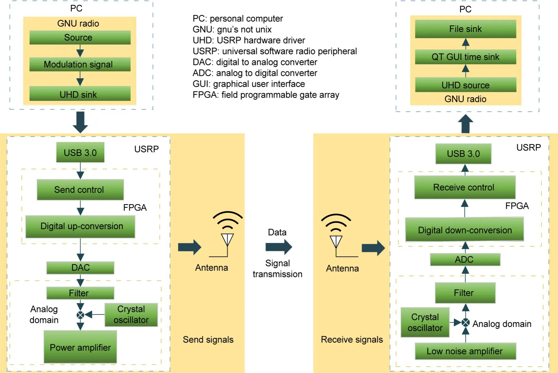
Fig.1 Architecture of the signal transceiver system

Flow graphs are constructed using gnu’s not unix(GNU) radio companion and a file source module is used to read the set signal data flow from the personal computer (PC).The data in the file source are pre-designed data of multiple modulation types.The modulation categories selected for this study are based on those previously used for radio datasets in modulation identification (O’Shea and West,2016).Modulation types are divided into analog modulation and digital modulation.Analog modulation includes double side band (DSB) modulation,simple side band(SSB) modulation,and frequency modulation (FM).Digital modulation includes 8 phase shift keying(8PSK),binary phase shift keying (BPSK),continuous phase frequency shift keying (CPFSK),Gauss frequency shift keying (GFSK),pulse amplitude modulation 4 (PAM4),16 quadrature amplitude modulation (16QAM),64 quadrature amplitude modulation(64QAM),and quadrature phase shift keying (QPSK).After sampling the modulated signal,the modulated signal can be expressed as

whereA(k) is the instantaneous amplitude of the signal,f(k) is the instantaneous frequency,andθ(k)is the instantaneous nonlinear phase.Using the trigonometric formula,we obtain

whereI(k) is the in-phase component andQ(k) is the quadrature component of the complex signal.Noise is added at different intensities for different kinds of modulated design signals.The SNR increases from-10 to 10 dB in 2-dB increments.The noised signal is as follows:

wheren(k) is the added noise.

2.2 Signal pre-processing

Our scheme adopts the pre-processing method of wavelet noise reduction for the received in-phase and quadrature data,and saves the multi-channel data and SNR labels of each modulation type.The processed data are directly fed into the deep learning network recognition model.

Wavelet threshold noise cancellation is a classical method in signal noise reduction (Donoho,1995).The wavelet transform originated from the Fourier transform,which convertes time domain functions to frequency domain functions by transforming them into trigonometric functions or their linear superposition (Harris,1978).The Fourier transform uses the entire signal in the time domain to extract spectral information,and obtains a single determined spectral value that does not reflect local characteristics.Compared with the Fourier transform,the wavelet transform chooses a finite-length family of wavelet functions (Chang et al.,2000).The family is obtained by translating and telescoping the wavelet basis,which decays rapidly to zero and integrates to zero in (-∞,+∞);i.e.,the amplitude oscillates between positive and negative.The essence of the wavelet transform is the inner product of the signal and the family of wavelet functions,i.e.,the projection of the signal onto the family of wavelet functions (Sendur and Selesnick,2002).The classical wavelet transform equation is as follows:

wheref(t) is the input signal,Ψ(t) is the wavelet basis function,ais the scale parameter that performs function scaling,andbis the translation parameter that changes the function action position.The result of the transformation reflects not only the frequency components contained in the signal,but also the corresponding time domain location.Most practical applications use discrete wavelet function families:

wherea=b=nb0,m,n∈Z,anda0＞1.The wavelet transform relies on differentmandnfor different resolutions,as well as different translations,to decompose the signal to different scales.Therefore,the wavelet transform can analyze the localization of non-stationary signals in the time–frequency domain.

We choose Daubechies’ wavelet basis function for the discrete wavelet transform.Daubechies’ wavelet belongs to compactly supported orthogonal wavelets.As a common function for signal decomposition and reconstruction,it has good regularity (Li B and Chen,2014).The Mallat algorithm carries out the decomposition,and the wavelet coefficients of low and high frequencies are

wherecj[k] is the low-frequency wavelet coefficient,anddj[k] is the high-frequency wavelet coefficient.The selected wavelet basis function determines the scale and wavelet coefficients.The number of decomposition layers isj,andNis the signal length.Most of the noise in the data is distributed in highfrequency details,and needs to be eliminated.A fixed threshold is used to remove noise (Jia et al.,2013).The formula for threshold selection is as follows:whereλis the selected threshold andwis the original wavelet coefficient.For the threshold function,the soft threshold selected for denoising is

wherewλis the wavelet coefficient after noise reduction.When the absolute value of the wavelet coefficients is greater than the given threshold,the wavelet coefficients subtract the threshold;when the absolute value is less than the given threshold,the wavelet coefficients are discarded.The wavelet inverse transform is performed on the filtered signal,i.e.,wavelet reconstruction.The equation is as follows:

The low-frequency coefficients and noise cancellation high-frequency coefficients are reconstructed,which can realize the pre-processing of wavelet noise reduction and obtain the estimated value of the recovered original signal.

3 Automatic modulation recognition system model

In this section,we first describe the overall framework of the signal recognition system and introduce the recognition network in the framework,i.e.,the deep adaptive threshold feature fusion network.We then provide detailed descriptions of two critical subnetworks of the recognition network: the deep adaptive threshold denoising network and the deep multiscale feature fusion network.

3.1 Overall framework of the signal recognition system

The overall framework of the signal recognition system is shown in Fig.2.The signal transceiver system collects the modulation signal to obtain in-phase and quadrature components.We use wavelet noise reduction on the components and combine them into multi-channel data.At this point,the data processing is completed.The pre-processed data are read into the deep adaptive threshold feature fusion network designed in this study to obtain a prediction.The symmetric cross-entropy loss function between the predicted category and actual category is calculated to obtain the loss value.The parameters are iteratively optimized according to the loss values to obtain the final recognition model.

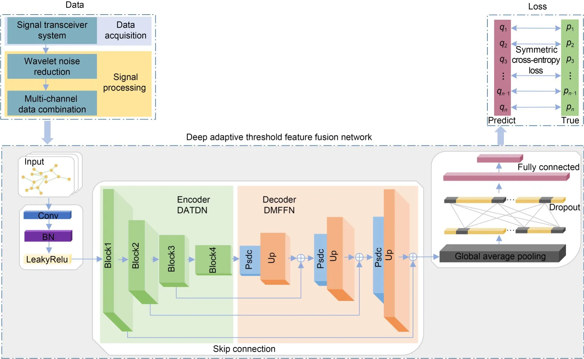
Fig.2 Signal recognition system framework

In the first step of the deep adaptive threshold feature fusion network,the input data are updated with dimensionality by the convolutional layer and pass through the batch normalization (BN) layer and LeakyRelu function.In the next step,the data pass through the critical components of the recognition network.The data are first extracted by the deep adaptive threshold denoising network of nonlinear encoding for feature extraction,and then dimensionally restored by the deep multi-scale feature fusion network of nonlinear decoding.We use the idea of an autoencoder to construct the above two sub-networks for modulation signal identification.We set four blocks with different dimensions in deep adaptive threshold denoising network with nonlinear encoder structure for feature extraction of different dimensions.Noise elimination means are introduced into each block.A threshold learning network with a designed threshold function removes redundant information from the set of learned features.This enables the network to automatically identify the noise to be removed and overcome the difficulty of determining the optimal value for setting the threshold manually.In the nonlinear decoding deep multi-scale feature fusion network,we set up decoding blocks corresponding to the dimension of the encoding block.In each decoding block,we convolve the input features using a parallel structure of dilated convolution for multi-scale feature extraction and superposition to form fused features and then upsample the fused features.The coding and decoding information is fused using skip connection so that the network learns both global and local information.Each decoding block is serially connected and gradually recovered to the initial data dimension.The output features go through a global average pooling layer,a dropout layer,and a fully connected layer to obtain the probability of each signal recognition.

3.2 Deep adaptive threshold denoising network

We propose a deep adaptive threshold denoising network based on the residual network.While ensuring the effectiveness of the network,this adaptively learns the threshold value and eliminates irrelevant data features to play the role of signal denoising.The deep adaptive threshold denoising network consists of four blocks of different dimensions,and each block contains a corresponding number of deep adaptive threshold denoising modules.The structure of each module is shown in Fig.3.The deep adaptive threshold denoising module contains an additional sub-module for setting the threshold of residual paths with respect to the deep residual module.The sub-module consists of a threshold training module and a threshold function.The threshold training module sets the corresponding threshold value for each channel feature.The threshold function can adaptively eliminate noise by judging the relationship between the data and the threshold of each channel.

Fig.3 Deep adaptive threshold denoising module

The core of the deep adaptive threshold denoising module lies in the design of threshold noise elimination for the residual path (Fig.3).Initial feature extraction is performed using the convolutional layer,BN,and the LeakyRelu function.Global average pooling then transforms featuresC×W×Hinto output featuresC×1×1 with global receptive fields,preventing overfitting and simplifying the computation when designing the subsequent noise elimination model thresholds.Among them,C,W,andHform a three-dimensional tensor,whereCrepresents the number of channels,Wrepresents width,andHrepresents height.After aggregatingC×W×Hinto the output features ofC×1×1,the model is divided into two parallel structures: one considers the relationship between different channels based on the original features,and the other is designed as the threshold training network.

The first path flattens the globally average pooled featuresxinto a one-dimensional tensor (C×onedimension),with each data value representing a feature within the current channel.Then the weights corresponding to each channel data value in the whole feature set are calculated by iterative optimization of the BN layer,Sigmoid function,and neural network propagation process.Each weight is multiplied by the feature value in the corresponding channel to obtain the feature containing the respective importance level.Compared with the direct output of features with the same weight,this method can better fit the dependency relationship between each channel and provide more critical information for subsequent network processing.

The other path is to obtain adaptive thresholds and use the threshold function to eliminate noise.Here,xis flattened in one dimension and multiplied with the features flattened by the adaptive local channel convolution.The resulting features are decompressed.Since the channel dimension is usually an integer multiple of 2,and considering the limitations of the linear mapping relationship for feature selection (Wang QL et al.,2020),an exponential function with a base of 2 is chosen to reflect the relationship between the convolution kernel and the number of channels.The adaptive local channel convolution is

whereKis the convolution kernel size,indicating how many close neighbors participate in the calculation of the specified channel.The sizes areγ=2,b=1,and convolution kernels are related to the number of channels in the current feature.ConsiderKconvolution kernels to capture local cross-channel interaction information,which can set thresholds for different channels by adaptive local cross-channel convolution.Input each channel data value and threshold value into the designed threshold function for adaptive noise elimination.The conventional threshold functions are hard thresholding and soft thresholding.The hard thresholding is

whereηis the set threshold value,xdenotes the input data,andxhdenotes the threshold noise elimination result.The hard threshold function is not continuous near the threshold value,causing the pseudo-Gibbs effect.Although the continuity of soft thresholding is improved,the sign function is prone to oscillate at the intermittent point,which affects the denoising effect.In our scheme,we use the tanh function instead of the sign function.The formula of the tanh function is

Fig.4 shows the difference between the tanh function and the sign function.

Fig.4 Function image

Compared with the sign function,the tanh function is smoother at the intermittent point,eliminating the effect of the optimization difficulty caused by the intermittent point of the sign function on the denoising process.In addition,the data whose absolute values are greater than the threshold when using soft thresholding have a constant deviation between the denoised value and the actual value,which affects the approximation of the denoised output and the actual data.Therefore,our designed threshold function is as follows:

whereζ1andζ2are the threshold results trained by adaptive noise elimination,xdenotes the input data,andxζdenotes the output of the deep neural network based on threshold function noise elimination.The network is flexible to self-learn the threshold value corresponding to the current feature so that essential features and redundant features learn different thresholds.Different noise elimination results are obtained by the threshold function.The features of the relationship between the adaptive noise elimination results and the retained channels are summed as the output of the residual path.This model ensures the overall efficiency.

3.3 Deep multi-scale feature fusion network

Our design uses a deep multi-scale feature fusion network as a decoder.The network consists of deep multi-scale feature fusion decoding blocks of different dimensions.Each decoding block corresponds to the dimension of the deep adaptive threshold denoising coding block.First,the decoding block synthesizes more discriminative features using continuous incremental multi-scale dilated convolutions for the input features.Dilated convolution is a method that increases the receptive field without adding additional computational effort (Wei YC et al.,2018).The receptive field is the size of the region where the extracted features are mapped to the input space (Rawat and Wang,2017).An increase in the receptive field indicates a larger spatial reach to the original data.Dilated convolution contains a hyperparameter dilated rate compared to standard convolution.Let the dilated rate bed.Thend-1 zeros are inserted between two adjacent elements of the convolution kernel,which constitutes a sparse filter:

wherenis the size of the equivalent convolutional kernel after expansion andkis the input convolutional kernel size.The output data size iso,iis the input data size,pis the padding size,andsis the step size.Compared with standard convolution,dilated convolution can obtain a denser feature response while learning fewer feature parameters.Fig.5 shows the dilated convolution parallel structure designed in this study.

Fig.5 Parallel structure of dilated convolution (References to color refer to the online version of this figure)

The parallel structure contains four-way dilated convolution with progressively increasing dilated rates.The light blue rectangular boxes in Fig.5 show the specific role of the dilated convolution layer for each way.In Eq.(15),assumingkis 3,we set the dilated rates in four ways to be 1,2,3,and 5.The change of each red box area represents the change in the size of the individual convolution kernel,so we can obtain the equivalent convolution kernel sizes to be 3,5,7,and 11,respectively.This expands the original action range of the convolution kernel and increases the receptive field.Meanwhile,the parallel incremental dilated convolution design can map the features of different sizes in the input features to the corresponding positions of the output features.After BN and the LeakyRelu function,the results are prepared for the next step of multi-scale fusion.To prevent the convolution kernel from degenerating into a filter of 1×1 and ignoring the overall features when the dilated rate increases,the module also parallels one-way global average pooling to restore global features.This way then goes through convolution to recover the channel dimension and upsampling to recover the size of the features.The designed five-way multi-scale parallel features are fused,and the features are subjected to 1×1 convolution,BN,the LeakyRelu function,and the dropout layer to obtain multi-scale fusion decoding features.

After the dilated convolution parallel structure,we use the bilinear interpolation method for upsampling calculation.Upsampling is a means of recovering data information.The four existing pixel values around the target point of the original image are used jointly to determine the target point’s pixel value.The core idea is to perform a linear interpolation in each of the two directions,which is computationally small and easy to implement.

Furthermore,the coding noise reduction feature and the decoding recovery feature of multi-scale analysis of the corresponding channel are skip-connected to obtain new features and then inputted to the next layer for continuous decoding.This process fuses high-level features with low-level features to obtain global and local information and mine the available information fully.

4 Experimental results and discussion

We verified the effectiveness of our network experimentally using the acquired data.

4.1 Dataset preparation

The baseband signal generated by the source is limited by the antenna size and the channel bandwidth.The signal has a low frequency,which causes significant attenuation and distortion when transmitted directly.Therefore,various modulation methods are needed to change the baseband signal into a form suitable for transmission on the corresponding carrier frequency.The dataset was the modulated signal obtained by using a software radio platform built by USRP to transmit and receive signals in a natural environment.It serves to support the next step to prove the practicality of the deep adaptive threshold feature fusion network.The 11 modulation types in this study were DSB,SSB,FM,8PSK,BPSK,CPFSK,GFSK,PAM4,16QAM,64QAM,and QPSK.Since the feature extraction recognition ability differs at different SNRs,noise was added to the modulated signal.The SNR ranged from -10 to 10 dB,increasing every 2 dB,producing signals at 11 SNRs.There were 1000 samples for each type of signal at each SNR,so the dataset contained 121 000 samples.The in-phase and quadrature matrices were transformed into a multi-dimensional matrix using wavelet decomposition,fixed threshold denoising,and wavelet reconstruction.The training and testing set data were divided according to an 8:2 ratio.

4.2 Experimental environment and parameter settings

The experimental platform consisted of a Windows version operating system,an E5-2680 v4 CPU processor,and an A4000 graphics card with 30.1 GB RAM and 16.9 GB video memory.Our proposed model was built and trained in the PyTorch framework,which is one of the powerful deep learning frameworks for Python.The cross-entropy function can indicate the degree of difference between the two types of variables (Kline and Berardi,2005).The smaller the crossentropy function value,the closer the distribution of the two categories of variables,and the larger the crossentropy function value,the more significant the difference between the two categories.When the cross-entropy function is used,the simple category classification is overfitted,but the complex category classification with noise is still underfitted.Therefore,it is necessary to choose a loss function suitable for handling complex category labels.We chose the symmetric cross-entropy function (Wang YS et al.,2019).We first calculated

where Eq.(17) is the formula for cross-entropy function,Eq.(18) is the formula for reverse cross-entropy function,p(x) is the true distribution,andq(x) is the predicted distribution.The combination of crossentropy and reverse cross-entropy constitutes the symmetric cross-entropy function:

whereαlcesolves the problem of overfitting the crossentropy loss function andβlrceimproves the robustness of noisy data and enhances the overall system performance.Further,the symmetric cross-entropy loss function is handled using label smoothing (Szegedy et al.,2016) to reduce the undesirable effects of forcibly learning the wrong category when the labels themselves have problems.Error tolerance was set for each type of modulation label:

whereεis a small constant.Label smoothing makes the probabilistic optimization objective of the loss function no longer 1 and 0,i.e.,1 becomes 1-ε,and 0 becomesε/(k-1),reducing the effect of overfitting and mislabeling on classification.To minimize the value of symmetric cross-entropy loss,the network needs to choose a suitable optimization strategy.Three gradient descent algorithms,SGDM,Adam,and RMSProp,were selected.The experimental results were recorded for every 4 dB increase from -10 dB to choose the most suitable strategy for this scheme.The results are shown in Table 1.

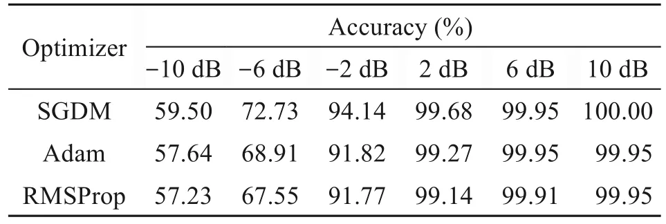
Table 1 Identification results of different optimization methods

A better optimization strategy can be obtained by using the SGDM method.SGDM is based on the SGD optimization algorithm but it incorporates a firstorder momentum update term.SGDM simulates the object’s inertia.The descent speed is increased for the position where the current gradient is consistentwith the last gradient.In other cases,the descent speed is reduced to avoid oscillation near a local optimum.This network uses SGDM for efficient learning of the network structure.At each SNR,we used the ratio of correctly classified signals to the total number of samples as the recognition accuracy for evaluating network performance.The confusion matrix of the modulated signals identified by the network was also plotted to evaluate the classification performance.For each class of modulated signals,TP means that the model correctly predicted signals,and FN means that the model incorrectly predicted signals as other classes.Thus,the prediction accuracy under each signal class is defined as

4.3 Network recognition results and analysis

Samples in the set were divided into 50 epochs.The batch size was set to 16.

4.3.1 Effect of network depth on experimental results

Under the network structure designed in this study,the number of deep adaptive threshold denoising modules in each coding block was changed to alter the number of overall network layers,to explore the influence of network depth on experimental results.The number of deep adaptive threshold denoising modules was increased one by one until optimal network architecture performance was obtained.The experimental networks included network A with 4 deep adaptive threshold denoising modules such that the numbers of modules from coding block 1 to coding block 4 were distributed as [1,1,1,1],network B with 5 modules such that the numbers were distributed as [1,1,1,2],network C with 6 modules such that the numbers were distributed as [1,2,1,2],network D with 7 modules such that the numbers were distributed as [1,2,2,2],network E with 8 modules such that the numbers were distributed as [2,2,2,2],and network F with 9 modules such that the numbers were distributed as [2,2,2,3].Fig.6 shows the experimental results of the six constructed depth networks at low SNRs of [-10,-2] dB.

Fig.6 Experimental results at different network depths

From the experimental results,when the number of deep adaptive threshold denoising modules was between 4 and 8,the recognition accuracy of the network under each SNR increased with the increase of the number of modules.This proved that as the depth of the network increases,the network learns richer feature information,expresses the features more strongly,and improves recognition results.When the number of modules increased from 8 to 9,the recognition accuracy of the network decreased under partial SNRs.The recognition accuracy was 59.50%,72.73%,and 94.14% at -10 dB,-6 dB,and -2 dB with 8 modules,respectively,and decreased to 58.32%,71.18%,and 93.41%,respectively,when the number of modules increased to 9.The reasons are as follows.First,the network dataset in this study was signal data,which do not need large-scale complex image feature recognition.Therefore,the recognition accuracy can easily reach saturation when the number of network layers rises.Second,the module parallelizes part of the hidden layer structure when the residual path is designed,accelerating the increase of the number of network layers.When the depth reaches the boundary value,increasing the depth again will gradually lose some shallow effective information and cause a decrease in accuracy.Additionally,the number of parameters of the network with 8 modules was 18 750 859,while the number of parameters of the network with 9 modules was 23 472 532.The increase in the number of parameters increases the training time.In this study,we combined the results of classification accuracy and model complexity.We selected network E containing 8 deep adaptive threshold modules such that the distribution of the numbers of modules from coding block 1 to coding block 4 was [2,2,2,2] for experiments.

4.3.2 Recognition results of feature fusion networks with different dilated rates

We tried to set different combinations of dilated rates for the parallel structure of dilated convolution in the decoding block.In the four-way parallel dilated convolution,we set the dilated rate to increase one by one.We chose the structures with four-way dilated rates of {1,2,3,5},{2,4,6,8},and {1,7,9,13} for the comparison experiment to select the most suitable combination of dilated rates under low SNRs.The results are shown in Fig.7.

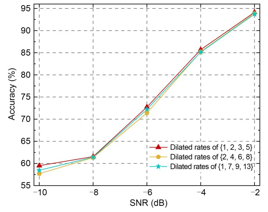
Fig.7 Identification results at different dilated rates

The results showed that using a structure with the dilated rate combination of {1,2,3,5} was better than using the two other structures,because the dilated rate directly determined the size of the receptive field.A combination with proportionally increasing dilated rates like {2,4,6,8} will lose the continuity of image information and form a gridding effect.When using a convolutional combination with dilated rates like{1,7,9,13} to process high-level information,a large convolution makes the input sampling sparse,resulting in local information loss.Therefore,the fourway structure with dilated rates of {1,2,3,5} was chosen for the network.

4.3.3 Identification results of the deep adaptive threshold denoising network based on multi-scale analysis

In this study,we set up a network with 8 deep residual modules such that the numbers of modules from coding block 1 to coding block 4 were distributed as [2,2,2,2] as the underlying framework network.For experimentation,we chose the underlying residual framework network,the deep adaptive threshold denoising network,the deep feature fusion network,and the deep adaptive threshold feature fusion network.The results shown in Fig.8 were used to verify whether the network designed in this paper improves recognition accuracy.

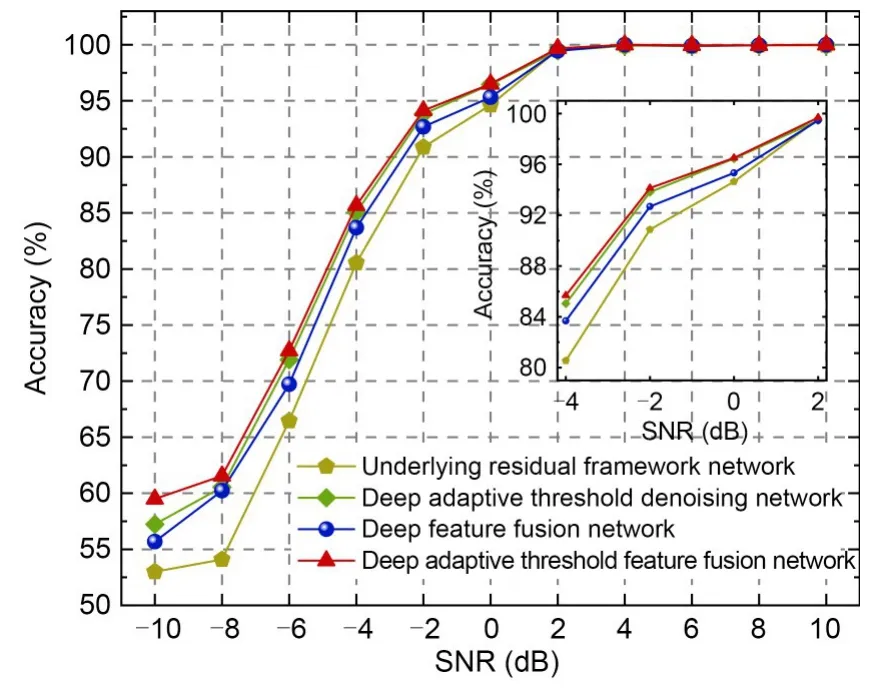
Fig.8 Results of the role of each network

The recognition accuracy of the designed deep self-learning threshold module was higher than that of the underlying residual framework.In particular,the feasibility of the threshold learning structure for redundant feature processing was well illustrated in the low SNR stage from -10 to -2 dB.The recognition effect of the deep feature fusion network with the addition of multi-scale analysis decoding was also better than that of the underlying residual framework.This indicates that the multi-scale incremental dilated convolutions based on our design achieve integration and interaction between the extracted features.The recognition results of the combined codec network outperformed the results of the above three networks,indicating that the network with the skip connection codec structure fully combines contextual data information.

4.3.4 Recognition accuracy comparison

The signal data were fed into the different networks under the same data pre-processing conditions for comparison with our network (Fig.9).

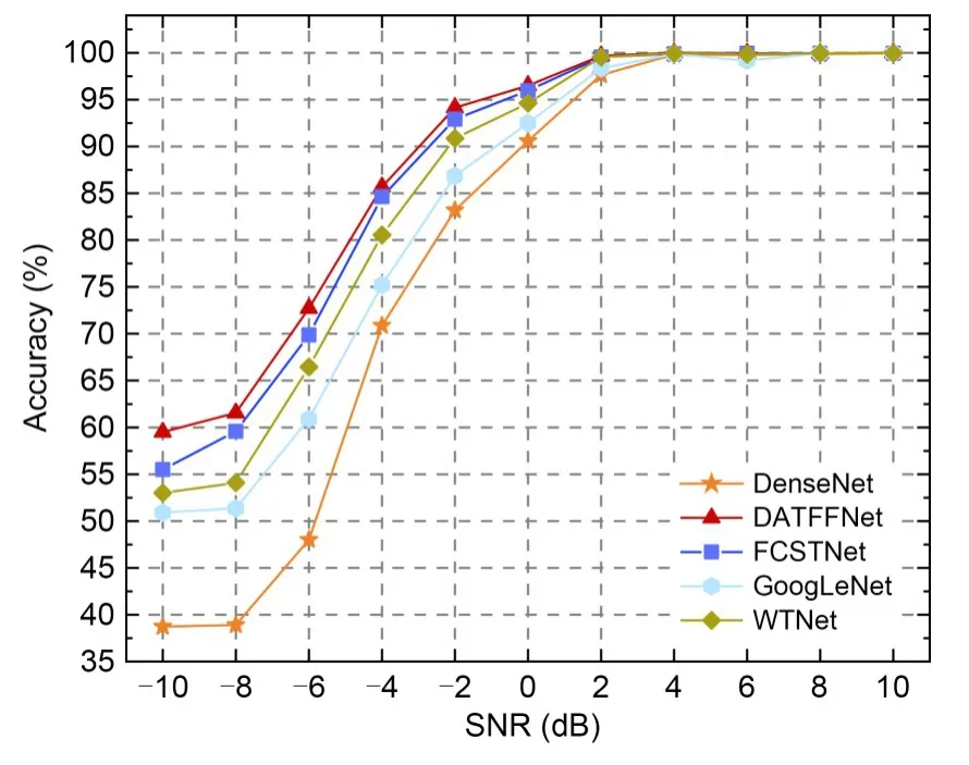
Fig.9 Different network modulation identification results

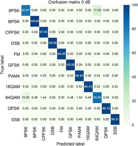
Fig.11 The 0 dB confusion matrix

Fig.12 The 10 dB confusion matrix

As SNR increased,the recognition accuracy of the five kinds of networks also increased.When SNR was lower than 0 dB,recognition rates changed significantly with the increase of SNR.When SNR was higher than 0 dB,the recognition rates increased slowly with the increase of SNR,and the final recognition rates tended to be stable.Under the overall SNR,the recognition accuracy of DATFFNet was higher than the accuracy of the other modulated classification networks.The recognition rate of DATFFNet reached 94.14% at -2 dB,which clearly demonstrates its superiority.We compared WTNet,FCSTNet,and DATFFNet.The recognition results obtained using the depth-based adaptive thresholding noise elimination method outperformed those of the traditional signal noise elimination method.In the low SNR stage,DATFFNet showed an accuracy improvement of 3.27%–7.45% compared with the traditional threshold noise elimination method,which shows the superiority of deep self-learning.Meanwhile,the noise cancellation effect of our thresholding module was better than that of using the fully connected layer combined with soft thresholding learning.In the low SNR stage,our network had an accuracy improvement of 1.05%–4%.The denoising method,which adaptively selectsKchannels,can effectively filter the irrelevant information while considering the direct correspondence between the channel and the weight to capture the most significant features of the signal.The overall recognition accuracy was higher,and the effect was better.We compared GoogLeNet (Szegedy et al.,2015),DenseNet (Huang G et al.,2017),and DATFFNet.The recognition results of our method were better than those of GoogLeNet for multi-scale aggregation in the low SNR stage,with an accuracy improvement of 7.27%–11.82%.This indicates the advantage of multi-scale information fusion and superposition in our design.In addition,the recognition results of our network were better than those of DenseNet for crosslayer connectivity.In the low SNR stage,the recognition accuracy of DATFFNet was significantly improved,which indicates the feasibility of cross-layer connection.

Visual analysis of the confusion matrix was carried out.Figs.10–12 show the classification results of the confusion matrix of the deep adaptive threshold denoising network based on multi-scale analysis when SNR was -10,0,and 10 dB,respectively.

The horizontal axis is the category predicted by the network,and the vertical axis is the actual category.The numbers in the table represent the probability that for the actual type corresponding to the vertical coordinate,the network predicts this type of signal as the corresponding type signal on the horizontal coordinate.At -10 dB,the recognition rates of most types of signals were above 60%,and the network model could roughly distinguish various types of signals.The recognition rates of 8PSK,16QAM,and 64QAM modulations were low,being 51.10%,41.88%,and 44.50%,respectively.At the lower SNR,the characteristics of these three types of signals and other types of modulation were not obvious,the similarity between the signals was large,and the probability of extracting ideal features was low,so the recognition rate was low.At 0 dB,the types of signals,except those of 8PSK and 64QAM,were only slightly confused,and recognition rates were higher than 95%,which proves that the network can distinguish these types well.8PSK had a 17.03% probability of being misjudged as 64QAM,and 64QAM had a 10.05%probability of being misjudged as 8PSK.In the results shown in Figs.10 and 11,a misjudgment always occurred between 8PSK and 64QAM.The reasons are as follows.First,in the process of network learning features,the features are selective,and the network easily loses part of the information,resulting in misjudgment between signals.Observing the recognition results of -10 dB and 0 dB,the recognition rates of 8PSK and 64QAM were lower than those of most other types,which explains that the features learned by this network caused 8PSK and 64QAM to be easily misjudged as other types.Second,when collecting data,the environmental noise seriously pollutes the 8PSK and 64QAM signals,and the parameters,such as the phase and frequency of the signals,are damaged,making it difficult to distinguish these two types.Hence,8PSK and 64QAM are always confused.At 10 dB SNR,a clear diagonal in the confusion matrix was achieved with a 100% modulation recognition rate for all modulation classes.From the three confusion matrix figures,the values on the main diagonal of the same type of modulation increased as SNR increased.This shows that the recognition rates of all kinds of signals increase with the increase of SNR,and the network recognition effect is gradually enhanced.

To further evaluate the performance of the algorithm,the RadioML2018.01A dataset (O’Shea et al.,2018) generated by the GNU radio was selected to test the algorithm.This dataset considers the effects of carrier frequency offset,symbol rate offset,delay time,and additive thermal noise on the signal in compromised environments.We selected 11 types of modulation signals,including 4ASK,AM-DSB-SC,AM-SSB-SC,BPSK,FM,GMSK,OOK,OQPSK,8PSK,16QAM,and QPSK.Different algorithms were inputted to the [-10,-2] dB segment for experiments,and the results are shown in Fig.13.

Fig.13 Recognition results of RadioML2018.01A

In impaired environments,the recognition of DATFFNet could reach 78.45% at -2 dB.Results of the algorithm used in our network were still better than those of the four other networks under low SNR,with an improvement of 0.32%–11.59%.This further proves that the designed network is suitable for noise threshold self-learning and multi-scale fusion analysis.

4.3.5 Model complexity of deep adaptive threshold denoising network based on multi-scale analysis

Model complexity is related to the computational resources used by the network.We used 1×1 convolution and adaptive grouping convolution to reduce the number of parameters.Further,we analyzed the experimental results from using different convolutional architectures in the encoding and decoding stages.Table 2 compares the number of parameters and recognition accuracy of the network using the underlying convolutional architecture of 1×n+n×1 in the encoding stage,the network using the output equivalent features ofn×nwithout expansion coefficients in the decoding stage,and our convolutional combination network,at low SNR.

Table 2 Numbers of parameters and recognition results of different convolutional architectures

Although the underlying architecture design of 1×n+n×1 reduced the number of parameters of the network,the recognition accuracy of the network was lower than that of our network.In multi-scale analysis,the training cost of using the convolutional network ofn×nwith no expansion was too large,and the recognition accuracy was not significantly improved.Therefore,the convolutional architecture of our proposed network not only had better recognition results,but also had fewer parameters and higher model efficiency.

5 Conclusions

In this paper,we proposed a deep adaptive threshold noise elimination network based on multi-scale analysis,called the DATFF network.First,unlike software simulation signals,our network uses USRP to build a software radio platform to transceive the actual signal and produce signal datasets.Second,we designed a coding network for deep adaptive threshold noise elimination to select the optimal threshold value in the denoising pre-processing stage.Meanwhile,we designed a deep multi-scale feature fusion decoding network and connected the coded and decoded features in skip connection.We conducted many comparative experiments on the collected datasets to demonstrate that our algorithm is effective in combining multi-scale information while eliminating noise from redundant features of signals,and has high recognition accuracy.In future work,we will focus on optimizing our network to achieve real-time classification using lightweight techniques while guaranteeing accuracy.We will also consider designing multi-path deep neuralnetworks to implement joint multi-task processing containing the automatic modulation recognition task.

Contributors

Xiang LI,Yibing LI,and Chunrui TANG designed the study.Xiang LI processed the data and drafted the paper.Yibing LI organized the paper.Chunrui TANG and Yingsong LI revised and finalized the paper.

Compliance with ethics guidelines

Xiang LI,Yibing LI,Chunrui TANG,and Yingsong LI declare that they have no conflict of interest.

Data availability

Due to the nature of this research,participants of this study did not agree for their data to be shared publicly,so supporting data are not available.