COPPER:a combinatorial optimization problem solver with processing-in-memory architecture*

Qiankun WANG ,Xingchen LI ,Bingzhe WU ,Ke YANG ,Wei HU ,Guangyu SUN,6,7,Yuchao YANG

1School of Software & Microelectronics, Peking University, Beijing 100871, China

2School of Computer Science, Peking University, Beijing 100871, China

3School of Integrated Circuits, Peking University, Beijing 100871, China

4Tencent AI Lab, Shenzhen 518057, China

5College of Physics and Information Engineering, Fuzhou University, Fuzhou 350116, China

6Beijing Advanced Innovation Center for Integrated Circuits, Beijing 100871, China

7Beijing Academy of Artificial Intelligence, Beijing 100080, China

Abstract: The combinatorial optimization problem (COP),which aims to find the optimal solution in discrete space,is fundamental in various fields.Unfortunately,many COPs are NP-complete,and require much more time to solve as the problem scale increases.Troubled by this,researchers may prefer fast methods even if they are not exact,so approximation algorithms,heuristic algorithms,and machine learning have been proposed.Some works proposed chaotic simulated annealing (CSA) based on the Hopfield neural network and did a good job.However,CSA is not something that current general-purpose processors can handle easily,and there is no special hardware for it.To efficiently perform CSA,we propose a software and hardware co-design.In software,we quantize the weight and output using appropriate bit widths,and then modify the calculations that are not suitable for hardware implementation.In hardware,we design a specialized processing-in-memory hardware architecture named COPPER based on the memristor.COPPER is capable of efficiently running the modified quantized CSA algorithm and supporting the pipeline further acceleration.The results show that COPPER can perform CSA remarkably well in both speed and energy.

Key words: Combinatorial optimization;Chaotic simulated annealing;Processing-in-memory

1 Introduction

Combinatorial optimization problems,abbreviated COPs,are prevalent but intractable in our daily lives.A classic COP is the traveling salesman problem (TSP),whose purpose is finding the shortest path through all cities and then back to the point of departure.Another COP we often meet is the work planning problem,which looks for an order of handling tasks to minimize the total timeout.Unfortunately,many COPs are non-deterministic polynomial complete (NPC).Consequently,we cannot solve them quickly when the problem size increases to a large scale.The prior theory proved that NPC problems can be transformed into each other in polynomial time (Karp,1972).In other words,we can simply pay attention to only one specific problem.

Many methods have been proposed to solve COPs.Though exact algorithms,such as enumeration and branch and bound,can obtain the optimal solution,they are usually extremely time-consuming.Approximate algorithms,such as the nearest neighbor algorithm for TSP,can obtain less acceptable solutions in polynomial time.However,they are normally designed for particular problems.Heuristic algorithms,which always focus on the thinking mindset to solve problems,are able to obtain decent but usually not optimal solutions in a specified time.However,none of the above methods can balance cost and performance well,especially when the scale of the problem is extensive.Machine learning has been proven to perform extremely well in many fields,so some works suggested applying it to COP,such as reinforcement learning (Mirhoseini et al.,2020),Hopfield neural networks(HNNs)(Hopfield and Tank,1985),and pointer networks(Vinyals et al.,2015).

HNN is a typical machine-learning-based method.HNN was proposed in the 1980s(Hopfield,1982).It is a type of fully connected recurrent neural network.Every neuron receives outputs from all other neurons and sends its output to all other neurons.An important property of HNN is Hamiltonian,or energy,which accounts for the stability of HNN.Starting with the initialized weights and neuron states,the energy of HNN keeps decreasing with computation until it reaches a minimum.

Hopfield and Tank (1985) proved that TSP could be solved using HNN.As shown in Fig.1,when solving a COP with HNN,we need to carefully map the energy of a network to the solution space of the COP.The mapping should ensure that the lower the energy,the better the corresponding solution to the problem.Therefore,we could obtain a sub-optimal/optimal solution when the HNN energy reaches a local/global minimum.

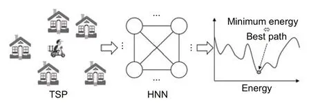
Fig.1 Solving the traveling salesman problem (TSP)with a Hopfield neural network (HNN)

However,because the HNN energy decreases only during computation,it is easy to get stuck at a locally optimal solution.Thus,avoiding the local optimal becomes the most challenging issue of the optimization problem.Therefore,Chen LN and Aihara (1995) proposed chaotic simulated annealing(CSA),making neurons in HNN receive not only outputs of other neurons but also their own outputs.The self-feedback will decay with time,so HNN should be chaotic at first and tend to stabilize gradually,which expands the exploration space and increases the probability of finding the global optimal solution.

Although the CSA method achieves great performance,it also suffers from the“memory wall” and low parallelism when it is processed on current processors.The processing-in-memory (PIM) architecture based on the memristor crossbar is a potential key to the dilemma.The memristor is an electronic device whose resistance can be adjusted,and it can be easily integrated into a crossbar to compute matrix-vector multiplication efficiently.Many works have applied the memristor PIM architecture to accelerate neural network computation(Chi et al.,2016;Shafiee et al.,2016;Song et al.,2017).Yang et al.(2020)suggested that the memristor PIM had the potential to implement a COP solver using CSA.However,the hardware architecture and many details of implementation,such as quantization and the design of the peripheral circuit,were not taken into consideration.Zhu et al.(2019) studied the quantization technique and PIM architecture design well.Zhu et al.(2019)focused on the multi-layer convolution neural network,while HNN is a fully connected cyclic neural network,so reanalysis is needed.Also,the previous PIM accelerators cannot directly perform CSA efficiently.Co-design of the algorithm and hardware is necessary.

In this paper,we propose an efficient PIM architecture,called COPPER,as the COP solver.COPPER is designed for CSA based on memristor crossbars.Thus,it can run a raw HNN naturally.Users just need to input the parameters of CSA,and COPPER will give an appropriate solution.Our main contributions are as follows:

1.We explore the influence that quantization brings to CSA,and determine the appropriate bit width.

2.We adapt CSA to hardware without reducing its performance.

3.We design an efficient COP solver with CSA and PIM,and propose a pipeline method.

Experimental results show that the speed and energy efficiency of COPPER are significantly better than those of CPU and GPU.

2 Preliminaries

In this section,we first provide the formulation of CSA and evaluate its performance.Then we introduce the memristor and PIM based on it.

2.1 Chaotic simulated annealing(CAS)

CSA is based on HNN,which is inspired by the Ising model (Cipra,1987).To explain the phenomenon of ferromagnetic phase transition in physics,Ernst Ising proposed the Ising model.In the Ising model,each neuron can perceive only the neurons adjacent to it.The Ising model succeeded in both physics and computer science.It was discovered that the Ising model could be used to solve the COP,as long as the problem is modeled suitably.Lucas(2014)showed the Ising formulations for many NP problems,most of which are COPs.

Different from the Ising model,HNN is a fully connected cyclic neural network,which means that each neuron can perceive all other neurons.The discrete HNN(DHNN)was proposed first,and the continuous HNN(CHNN)was proposed years after.The former can be used as content-addressed memory,and the latter can be used as a COP solver.Although CHNN is a little different from the Ising model,the formulations for COPs used by Lucas(2014)can also be applied to CHNN.Because each neuron can directly perceive more neurons,CHNN can achieve a better solution in fewer iterations.

CHNN is also troubled by local minima,so Chen LN and Aihara(1995)suggested adding self-feedback to CHNN,which is CAS.Here we use the symbols of Chen LN and Aihara (1995)to describe CSA.As shown in Fig.2,every neuronihas stateyiand outputxi,and is influenced by the biasIi.There is a connection weightwijbetween any two neuronsniandnj,andwij=wji.The formulation of CSA is

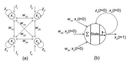
Fig.2 Chaotic simulated annealing (CSA) (a) and its neuron (b)

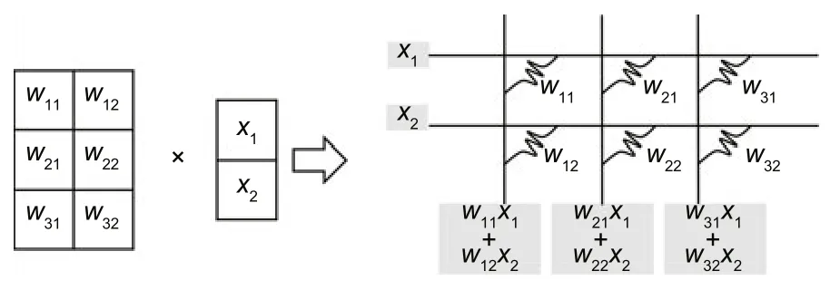
Fig.3 Memristor crossbar for multiplication

where∈,k,α,β,andI0are constants,andziis the self-feedback coefficient of neuroni.The original CHNN has no self-feedback;that is,zi=0.At every tick,every neuron updates its own state and output according to Eqs.(1)–(3).The order of neuron operation is not essential.All neurons can run asynchronously or synchronously in any order.

CSA has the same energy representation as the CHNN,which is shown in Eq.(4).It can be proved that without self-feedback (like the original HNN),the network energy will gradually decrease with time.When the self-feedback coefficients are not zero,the energy change direction of the network is unpredictable,namely chaotic.After the self-feedback coefficients are all zero,the energy decreases until reaching a local minimum or the global minimum.That is the reason why it is called CSA.

2.2 CSA performance

Here we test the CSA performance on TSP.To solve TSP,we need to model the problem.Assuming that there arencities in all,ann×nbinary matrixXrepresents a path we choose.InX,xij=1 means that the salesman will visit cityiat thejthposition.Therefore,the constraints consist of two parts:

1.Hard constraint: any position corresponds to one and only one city;any city corresponds to one and only one position.

2.Soft constraint: the shorter the path length,the better the path.

Now we give the whole constraint,that is,

wheredikrepresents the distance between cityiand cityk.The first part of the right-hand side of Eq.(5)is the hardware constraint,which should be zeros whenXrepresents a feasible solution.The second part is the software constraint,which should be smaller when the solution is better.By adjustingW1andW2,we can indicate whether we prefer to obtain a feasible solution or a better solution.

By matching the coefficients of everyxin Eqs.(4) and (5),we can compute the values ofwijandIineeded by CSA,and then perform calculations according to Eqs.(1)–(3).CSA will return a solution after reaching stability.The initial state can be set randomly.

We evaluate the performance of CSA on different numbers of cities.Positions of cities are generated randomly,and coordinates are in 0–1.Table 1 shows the constant parameters we set to test the performance of CSA.For problems of different scales,weuse different constant parameters.Constant parameters used in the problem with 10 cities are from Yang et al.(2020),and we fine-tune constant parameters for the others.As the number of cities increases,we tend to obtain feasible solutions (by decreasingW2)and increase the amount of annealing (by decreasingβand increasingz0) to explore a larger solution space.

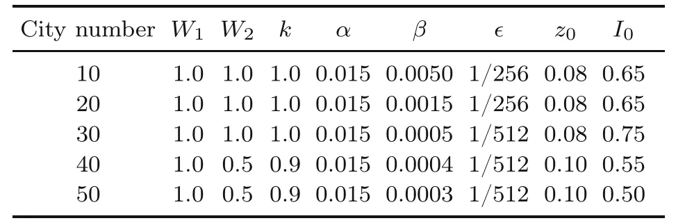
Table 1 Constant parameters used in chaotic simulated annealing when solving the traveling salesman problem

Table 2 shows the results.The best paths are obtained using Concorde,which is typical software to solve TSP.For each scale,we apply CSA 100 times and the simulated annealing (SA) algorithm 100 times for comparison.For fairness,we set different annealing rates for SA so that the amount of annealing approximately equals the number of iterations of CSAs.We show the best and average path lengths found by CSA and SA.

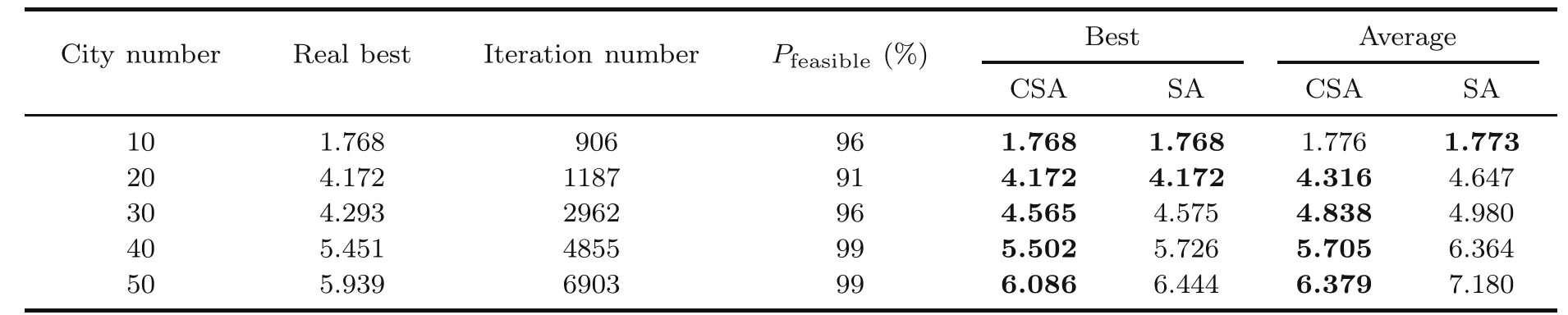
Table 2 Performance of chaotic simulated annealing (CSA) and simulated annealing (SA)

According to Table 2,CSA needs multiple iterations to reach the stable state,and it does not always obtain a feasible solution.As for the quality of the solution,CSA is better than SA.In fact,the solution quality is still not as good as that in Chen LN and Aihara (1995),because we do not spend much time in adapting the constant parameters.However,we can see that CSA can obtain good solutions,although the scale of the problem increases.

2.3 Memristor-based processing-in-memory architecture

Because CSA is fully connected,the amount of computation required will increase rapidly,which is not something that current general-purpose processors can handle easily.In fact,many neural networks are troubled by such extensive computation.Too many calculations are needed,although most of the calculations are similar.Therefore,PIM is proposed which intends to perform some simple operations in memory.PIM is created with a high degreeof parallelism and does not require much time for fetching data.

Yang et al.(2020)attempted to implement CSA using a memristor crossbar.In this work,the weights and self-feedback coefficients were written into the memristor cells,and other operations were simulated.The results showed that the memristor crossbar can perform CSA correctly.In addition,this work explored the convergence when selffeedback coefficients decayed with linear,exponential,and long-term depression,separately.However,the programming of the memristor cell is timeconsuming (Chen JR et al.,2020),so the time cost will increase rapidly if the memristor cell is adjusted frequently.The aim of Yang et al.(2020)was to verify the feasibility,so many practical problems,such as hardware architecture,scale,and algorithm quantization,were not taken into consideration.In the following sections,we will address these problems.

3 Algorithm

In this section,we first quantize CSA and find the proper bit width.Then we propose schemes to adapt CSA to hardware implementation.Finally,we evaluate the performance of the quantization and schemes on the max-cut problem.

3.1 Quantization

Quantization is necessary before implementing CSA on special hardware.Because matrix-vector multiplication is deployed on memristor crossbars,quantization of the weight and output should be taken into consideration.We analyze the influence of quantization by solving a 30-city TSP 100 times.The positions and constant parameters are the same as in Section 2.2.We pre-calculate float32 weights with float32 position coordinates and then quantize the weights into different bit widths for subsequent computing.Here we use symmetric uniform quantization,which is easy to implement.

Fig.4 shows the influence of quantization of the weight and output.The solid line represents the ratio between the path lengths of float CSA and quantized CSA.The dotted line represents the rate of obtaining a feasible solution.An interesting note is that quantized CSA sometimes obtains better solutions(the length ratio of float path to quantized path ＞1),which may be owing to the randomness.We can see that CSA is more sensitive to the quantization of the weight than to that of output.A weight of low bit width may incur a high failure ratio and solutions with bad performance.

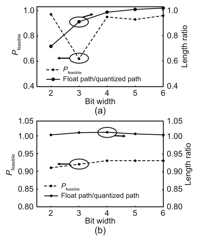
Fig.4 Quantization influence: (a) weight quantization;(b) output quantization

We think that the weight determines the trend of the network energy change.After the weight is quantized with too few bits,the network cannot obtain the right direction in every iteration,so it will fail at last.In addition,fewer bits erase the gap between a longer and a shorter distance,so the network cannot perceive the better path.According to Fig.4,we suggest using 4 bits for the weight.The finer the output granularity,the more the states that each neuron can have,and the larger the space that the entire network can explore.Also,CHNN and CSA have richer dynamic characteristics,which increase their adaptability.Therefore,we suggest using 8 bits for the output.The following subsections are based on 4-bit weight and 8-bit output.

3.2 Adaptation

We will propose some schemes in this subsection to adapt CSA to hardware.

The implementation of the sigmoid function is very expensive.Fortunately,fewer bits are enough for the output according to Section 3.1,so we could use a lookup table(LUT) to reduce the cost.

Because the output of the sigmoid is between 0 and 1 and we use 8 bits to represent the output,the input of sigmoid,assumed to bea,needs only to be between-5.54 and +5.54.According to Eq.(1),we havea=y/∈.We can specify∈as-ppower of 2,which does not influence the performance of CSA,so the division could be transformed into a shift.Note that we do not changeybut just use it to calculatea.The resultawill be truncated into 8 bits and be used as the sigmoid LUT.Therefore,Eq.(1) could be replaced by

In addition,zdecays exponentially in Eq.(3),which is not hardware-friendly.We can replace exponential decay with linear decay.That is,Eq.(3)could be replaced by

We apply the adaptation to the 30-city TSP.As shown in Table 3,linear decay has little effect on the algorithm.

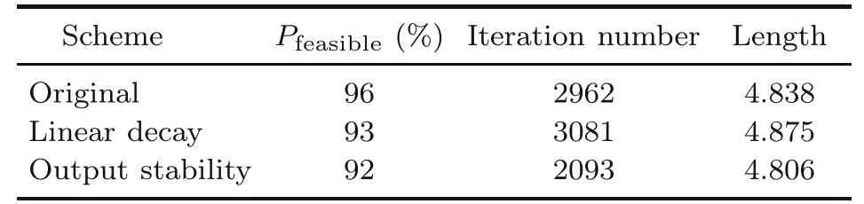
Table 3 Influence of the adaptation

Eq.(2)could also be transformed into

Although it seems typical,we do not fuse the self-feedback and weight,because modifying the weight,represented by the conductance of a memristor,takes a lot of time.

Another problem we need to consider is discontinuing computation in time after the network becomes stable.The stability of the network means that every value does not change again,including the energy of the network and the states and outputs of neurons.According to Eq.(4)or(5),the calculation of energy is especially complex,so we prefer using output as the criterion.To reduce the overhead of comparison between the last and the current outputs,we suggest just contrasting their highest bit.This is not absurd,because the final outputs always converge to 0 or 1.We believe that if the outputs do not change 10 times in a row,the network becomes stable.According to Table 3,the results of comparison between rounding values can represent the raw results very closely.In addition,it is shown that using output rounding values can evidently reduce the number of iterations,because the redundant iterations just change the output from＞0.5 to 1.0 in most cases.

3.3 Performance on the max-cut problem

CSA can solve many COPs directly as long as the energy function is suitably constructed.Also,many COPs can be transformed into each other,so CSA can also solve COPs indirectly by transforming them into those that can be solved.

To evaluate the feasibility of CSA and the above schemes on other COPs,we carry out experiments on the max-cut problem,which is also an NPC problem.The max-cut problem is to divide the node set of a graph into two complementary subsets so that the number of edges between the two subsets is maximum.Assuming that the graph includesnnodes,the following formulation can be used to evaluate a segmentation:whereiandjrepresent the nodes.aij=1 if nodeiconnects with nodej;aij=0,otherwise.xi ∈{0,1}reflects the subset node to whichibelongs.

According to Eq.(9),the energy function of the max-cut problem is as follows:

By building a Hopfield network ofnnodes,and comparing Eqs.(4) and (10),we can see thatwij=-4aijandIi=

Fig.5 is a graph whose edges are randomly generated.Fig.5 also shows one of the optimal segmentations,and the number of edges that are cut through is 12.We evaluate CSA with different schemes 100 times,and the results are shown in Table 4.The constant parameters in the experiments are consistent with those in the previous TSP problems of 10 cities.Weights and outputs are quantized with 4 and 8 bits,respectively.Obviously,when using various schemes,CSA can still solve the max-cut problem well.

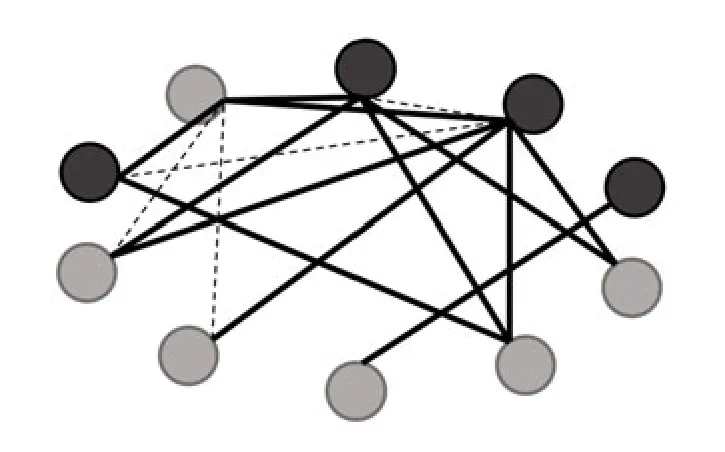
Fig.5 Max-cut problem

4 Architecture design

4.1 Overview

COPPER is composed mainly of a subprocessor-element(subPE)array and peripheral circuits,as shown in Fig.6.Each subPE can calculate matrix-vector multiplication independently.The peripheral circuit,responsible for the parts except for matrix-vector multiplication,is implemented using traditional CMOS circuits.With the increase of the scale of CSA,the scale of subPE increases in the square while the peripheral circuit increases linearly.That is,each column of subPE is equipped with one peripheral circuit.COPPER covers only the operation of the network,so the calculation of weights is the concern of the host.In consideration of the sign of parameters,the weights may need equivalent linear transformation to make them all non-negative numbers.This was discussed in Yang et al.(2020).

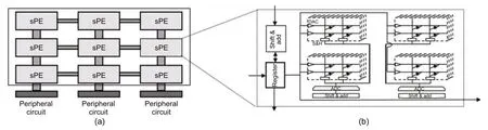
Fig.6 COPPER overview (a) and subPE (b)

After parameters are written,COPPER starts running until the network stabilizes or reaches the upper limit of the cycle.During operation,data will be transmitted between subPEs.Specifically,a subPE communicates from left to right and from top to bottom,which can save the bandwidth between the subPE and buffer.The pipeline between the subPE and peripheral circuit can save time,and the delay of the peripheral circuit is covered by the subPE.

4.2 SubPE

Each subPE has 16 128×128 memristor crossbars,digital-to-analog converters(DACs),analog-todigital converters (ADCs),sample-and-hold (S+H)devices,registers,and shift-and-add(S+A)units.

Due toIRdrop,thermal noise,random telegraph noise,and so on,memristor crossbars may not always work ideally,which will result in computing errors.It is not mature to write a 4-bit weight into just one cell,which may lead to more errors.However,with the help of the compensation circuit and other means,memristors composed of single-bit cells can run stably.In Hung et al.(2022),the systemlevel inference accuracy of a ResNet-20 model did not decrease at all.Therefore,we split one 4-bit weight into four cells.Similarly,we divide one input into 8 bits and send one bit into the crossbar at a time,because using an 8-bit DAC is risky.In this way,one bit of the input produces 4 bits,which should be put in appropriate positions,separately.One input produces eight groups of outputs,which should be shifted and accumulated.In fact,this is the same as the column multiplication of binary multiplication.In a word,we spend more time on inputs and more hardware on weights,but achieve perfect stability.

Because each row of subPEs shares the same input,we make each subPE receive the input from left and immediately transmit the input to the subPE on right.The leftmost subPE obtains data from the data line.Because the results of each column of subPEs will be accumulated together,we make each subPE receive the result from top,accumulate it in its own result,and send the new result to the subPE below.The results received by the uppermost subPE are all zeros.Therefore,we can use different numbers of subPEs to adapt to problems with different scales.

4.3 Peripheral circuit

The peripheral circuit starts after subPEs provide the result.In detail,the peripheral circuit will complete the remaining computation and judge whether the network reaches stability.Fig.7 shows the main data path of the peripheral circuit.As mentioned in Section 3.2,we make self-feedbackzdecay linearly and replace the sigmoid function with LUT.The final results arext+1,yt+1,andzt+1.We use the highest bit ofxtandxt+1for comparison to confirm that the network is stable.

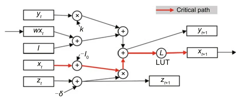
Fig.7 Peripheral circuit data path (References to color refer to the online version of this figure)

4.4 Pipeline

Because each iteration of CSA depends on the results of the previous iteration,it seems that there is no way to pipeline.However,considering the possible failure of CSA and the fact that the optimal solution cannot be obtained every time,we may need to run CSA several times to obtain an excellent solution for a particular problem.Therefore,we can run two CSAs for one problem at a time,without the CSAs interfering with each other,which is a pipeline not for different iterations in the same network but for different networks.

Specifically,for the same problem,the weight and bias are exactly the same,but the initial state is different,so we do not need to rewrite the weight and bias.We can write the first batch of the initial statey1(t=0),calculatex1(t=0),and putx1(t=0)into subPEs.After obtainingwx1(t=0),we input the second batch of the initial statey2(t=0),calculatex2(t=0),and putx2(t=0) into subPEs.At the same time,we usewx1(t=0) to calculate a newy1(t=1),so we can realize the pipeline.By simply incurring some costs to store two sets of constant parameters,we can obtain twice solutions in the same amount of time.

5 Evaluation

5.1 Experiment setup

Because there is no work designing a special hardware architecture for CSA,we compare COPPER with the general CPU and GPU processors.For TSPs with different numbers of cities,we run CSA on CPU and GPU,and estimate the energy cost and speed.The CPU is Intel®CoreTMi7-6700K CPU@ 4.00 GHz with 32 GB RAM,GPU 1 is NVIDIA GeForce GTX 1080 Ti,and GPU 2 is NVIDIA A100 80 GB.We use the Python packages pyRAPL and pynvml to estimate the cost of CPU and GPU,respectively.As for COPPER,we use 10× 10 subPEs,which can solve a 50-city TSP,in evaluation.The parameters in Table 5 are from Shafiee et al.(2016).

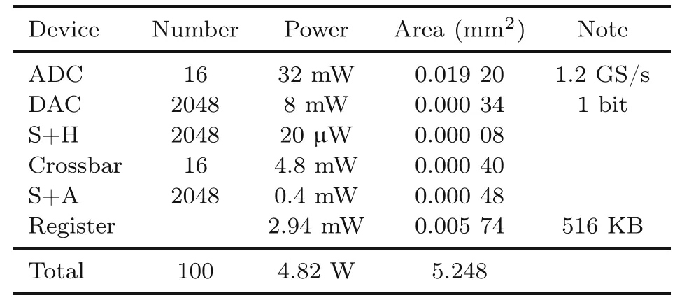
Table 5 Device parameters

Obviously,as the scale of the problem increases,the workload of peripheral circuits increases linearly,while the subPE sustains square growth.As shown in Table 5,each column of subPEs could obtain no more than 256 products in 1.2×2-21s.It is enough for the peripheral circuit to perform 256 times in 1.2×2-21s.That is,the frequency should be 600 MHz.The critical path(shown as the red line in Fig.7)contains two additions,one multiplication and an LUT,so the peripheral circuit can easily reach 600 MHz.Therefore,matrix-vector multiplication is the main bottleneck,and COPPER does not require high-speed peripheral circuits,so we focus only on the comparison of matrix-vector multiplication.

5.2 Speed

We run CSA 10 000 times and compute the average time cost on CPU and GPU.According to Table 6,as the scale of the problem increases,the acceleration of COPPER becomes obvious.

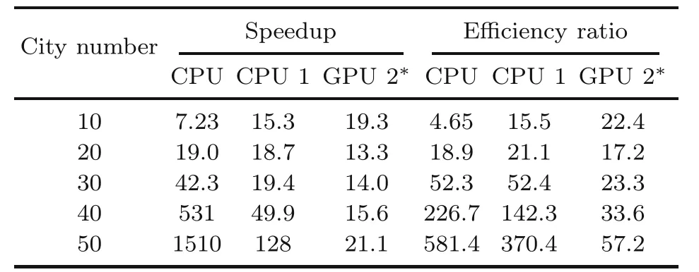
Table 6 Comparison of COPPER with CPU and GPU

The practical speedup should not be as significant,because many details,such as communication,buffer,and synchronization,are not taken into consideration.However,the obvious speedup is predictable due to the significant reduction in communication,and the bigger the scale,the more obvious the speedup.

5.3 Energy efficiency

We run CSA 10 000 times and compute the average energy cost on CPU and GPU.For CPU,the Python package pyRAPL can directly estimate the energy cost of the selected codes.For GPU,the Python package pynvml can monitor the real-time power,and we calculate the energy by multiplying the power and time used.

As shown in Table 6,COPPER is much more efficient than CPU and GPU.With the increase of the problem scale,the improvement of efficiency is more and more obvious.We think that there are two main reasons.First,we assume that all subPEs are running,even if the problem scale is not enough touse all crossbars,so the bigger the problem,the better it is for COPPER.Second,with the increase of the problem scale,general-purpose processors spend much more energy on data handling and cyclic calculation,while COPPER holds the calculation in memory,which significantly reduces the energy cost.

5.4 Comparison with SA

Although COPPER can implement CSA effi-ciently,it is necessary to compare COPPER with other algorithms on general-purpose processors.Here,we test the time and energy cost of SA algorithm on CPU.Because the SA algorithm is not computation-intensive,GPUs are not in the test.The SA setup is the same as in Section 2.2,and its time and energy are still from the Python package pyRAPL.The time of CSA on COPPER equals the average iteration number divided by the frequency of COPPER,and the energy equals the value of the time times the power.Note that the energy of the peripheral circuit is ignored because this is negligible (Li et al.,2022).

Table 7 shows the results.Compared with SA on the CPU,COPPER still exhibits clear speedup but fails in energy.The reason is that CSA contains a lot of computation(matrix-vector multiplication),while SA does not.COPPER reduces the time by parallel computing,while the energy needed is still so much.However,according to Tables 2 and 7,COPPER has advantages in speed and quality of the solution,so it is very competitive.

Table 7 Speed and efficiency of CSA compared to those of SA

6 Related works

The Ising model was proposed for the phenomenon of ferromagnetic phase transition in physics.It regards the object as ad-dimensional lattice,and each lattice site represents a small magnet.Adjacent magnets interact with each other,which could be considered as coefficients/weights.The whole system has a Hamiltonian/energy,which is related to weights,magnet properties,and external magnetic fields.

After it was discovered that the Ising model could be used to solve COPs,a series of hardware was designed,such as quantum annealing (Johnson et al.,2011;Shin et al.,2014) and CMOS annealing (Yamaoka et al.,2016;Takemoto et al.,2019,2021;Yamamoto et al.,2020).They all strived to simulate more and more lattice sites to solve problems on a larger scale,and Takemoto et al.(2021)even implemented 1.44×105lattice sites.To escape from local minima,these designs introduced various annealing mechanisms.For example,Yamaoka et al.(2016) and Takemoto et al.(2019) made the state of spin,corresponding to the small magnet in the Ising model,inverse randomly,while Takemoto et al.(2021)used probabilistic inversion.In addition,they equipped tens of thousands of spins to handle large-scale problems.

7 Conclusions and discussion

To solve combinatorial optimization problems,we improve the chaotic simulated annealing algorithm and design COPPER.COPPER uses advanced storage technology to improve the parallelism of operation and obtains great performance in power consumption and speed.COPPER is scalable and can solve large-scale COPs.In addition,COPPER can not only run chaotic simulated annealing,but also support the original continuous Hopfield neural network for other applications.

However,we also see that the Ising model,CHNN,and CSA all require a high degree of parallelism,while the current hardware does not support reuse,so the hardware scale must increase with the increase of the problem scale.Physically,the hardware scale cannot increase without limits.So far,the biggest ReRAM nonvolatile PIM macro has been 8 Mb (Hung et al.,2022).Using one such macro,we can solve the TSP with 37 cities at most when quantizing the weights into 4 bits.Furthermore,using more macros,TSP with more cities can be solved.Meanwhile,except for the development of hardware,supporting temporal reuse of hardware or implementing CSA using quantum may be a promising direction.

Contributors

Qiankun WANG led the research and was mainly responsible for implementing the algorithm,designing the hardware,and drafting the paper.Xingchen LI provided the design ideas and some data for the hardware part.Bingzhe WU sorted out the algorithm and pointed out the possibility of combining software and hardware.Ke YANG and Yuchao YANG laid the foundation for this research and provided some parameters for the algorithm.Wei HU provided the stability analysis of ReRAM and the latest research progress of ReRAM PIM macro.Guangyu SUN made many suggestions on the research,and revised and finalized the paper.

Compliance with ethics guidelines

Qiankun WANG,Xingchen LI,Bingzhe WU,Ke YANG,Wei HU,Guangyu SUN,and Yuchao YANG declare that they have no conflict of interest.

Data availability

The data that support the findings of this study are available from the corresponding author upon reasonable request.