一类基于不确定理论的分位数回归模型
2022-12-07 14:01:48李天用胡锡健
新疆大学学报(自然科学版)(中英文) 2022年5期
李天用,胡锡健
(新疆大学数学与系统科学学院,新疆乌鲁木齐 830017)
0 Introduction
Quantile regression is a method to obtain parameter estimates by minimizing the sum of the absolute values of the weighted residuals. Since 1978, when Koenker and Bassett[1]first introduced the concept of quantile regression, it has attracted the attention of many scholars and has been widely used in various fields,such as data processing,systems engineering and probability statistics. Eide and Showalter[2]used quantile regression to study the effect of education on intergenerational income,this method is less restrictive on the random disturbance term in the model and reduces the cost of the experiment.Beirlant and Goegebeur[3]modeled in data processing by Pareto index, this model can estimate extreme quantile problems and effectively analysis the tail weights on the conditional distribution of response variables. Somers and Whittaker[4]applied the quantile regression into retail credit risk assessment practices,solutions at different quartiles can reasonably explain the different distributions in the financial services industry. Nikolaou[5]analyzed the effect of different magnitude shocks on the real exchange rate based on semi-parametric and non-parametric quantile regression models,which clearly reflect the pattern of exchange rate changes at extreme quantile. Yu and Moyeed[6]introduced the idea of Bayesian quantile regression and proved the robustness of quantile regression to heteroskedasticity. Tang and Kong[7]applied the idea of quantile regression to the linear semi-parametric model of functional data. Sun[8]further introduced the idea of quantile regression into functional data and established a functional data quantile regression model. He, Yan and Xu[9]combined the support vector integral quantile regression method with fuzzy information granulation to construct a quantile regression model based on fuzzy information granulation and support vector.
To the best of our knowledge,the quantile regression has been proposed usually in the framework of probability theory.Because the traditional quantile regression methods all assume that we have a large number of precise observations, and some observations are imprecise within a certain range, e.g. height around 1.8 m, distance from the school building about 500 m, weight of the dog between 10 and 20 kg, etc. So, the results of the regression analysis method under probability theory will have a large bias, we need to use experts’ estimated imprecise data. Based on the above research background and problems,Liu[10−11]proposed uncertainty theory to fill these gaps and widely applied into various fields such as uncertain programming[12], uncertain calculus[13], uncertain statistics[14]and uncertain differential[15]. At the same time, Liu and his students put forward the principle of uncertain least squares method,the parameters were also estimated using experimental data and the sum of squares of distances from uncertain distributions[14].They also introduced point estimates of the unknown parameters in the uncertain multiple regression model[16]. Shortly after, Lio and Liu[17]made interval predictions of the response uncertain variables to determine the range of values of the estimates. Ye and Liu[18]derived uncertain least squares estimates of the unknown parameters,in which the disturbance terms are assumed to have normal uncertainty distributions.Liu and Yang[19]applied the least absolute principle into the estimates of the unknown parameters in an uncertain multiple regression model. To further improve the uncertainty theory, this paper develops an uncertain quantile regression (UQR)model based on previous studies combining quantile regression model and uncertainty theory. From the data perspective,using uncertain data can make the estimation results more accurate. From the model perspective,UQR can not only measure the effect of regression variables at the center of the distribution,but also fit the curves corresponding to different quantiles,which can analyze the characteristics of the data more comprehensively.
The rest of the paper is organized as follows. Section 1 reviews the basics of uncertainty theory. Section 2 defines the concepts of uncertain quantile and uncertain loss function. In Section 3, the UQR model is introduced. The uncertain parameter estimates,residual distributions and confidence intervals of the response variables are also obtained. In Section 4,numerical simulations are performed to compare the mean square errors of the original data and the uncertain data,and the robustness of the UQR model is demonstrated. The conclusions are given in Section 5.
1 Preliminaries
In this section,we introduce some fundamental concepts and theorems based on uncertainty theory,including uncertain measure,uncertain variable,uncertainty distribution,uncertain expected value and uncertain variance.
Definition 1[10]Let L be a σ-algebra on a nonempty set Γ. A set function M : L → [0,1] is called an uncertain measure,if it satisfies the following axioms:
Axiom 1(Normality Axiom)M{Γ}=1 for the universal set Γ.
Axiom 2(Duality Axiom)M{Λ}+M{Λc}=1 for any event Λ.
Axiom 3(Subadditivity Axiom)For every countable sequence of events Λ1,Λ2,···,we have
Axiom 4(Product Axiom)Let(Γk,Lk,Mk)be uncertainty spaces for k=1,2,···. Then the product uncertain measure M is an uncertain measure satisfying
where Λkare arbitrarily chosen events from Lkfor k=1,2,···,respectively.
Definition 2[10]An uncertain variable ξ is a measurable function from an uncertainty space(Γ,L,M)to the set of real numbers,i.e.,for any Borel set B of real numbers,the set

is an event.
Definition 3[11]The uncertain variables ξ1,ξ2,···,ξmare said to be independent if
for any Borel sets B1,B2,···,Bmof real number.
Theorem 1[14]Let ξ1,ξ2,···,ξnbe independent uncertain variables with regular uncertainty distributions Φ1,Φ2,···,Φn,respectively. If the function f(x1,x2,···,xn) is strictly increasing with respect to x1,x2,···,xmand strictly decreasing with xm+1,xm+2,···,xn,then the uncertain variable
is an uncertain variable with inverse uncertainty distribution

Definition 4[10]Let ξ be an uncertain variable. Then the expected value of ξ is defined as
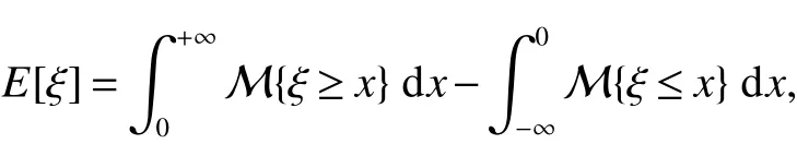
provided that at least one of the two integrals is finite.
For an uncertain variable ξ with regular uncertainty distribution Φ(x),its expected value can be obtained by

Theorem 2[14]Let ξ and η be independent uncertain variables with finite expected values. Then for any real number a and b,we have

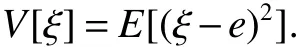
Definition 5[10]Let ξ be an uncertain variable with finite expected value e. Then the variance of ξ is defined by
For an uncertain variable ξ with regular uncertainty distribution Φ(x) and finite expected value e, its variance can be obtained by

2 Uncertain Quantile
The core of the quantile regression model is the quantile in probability theory. In order to build the UQR model, we define the concepts of uncertain quantile and uncertain loss function as follows.
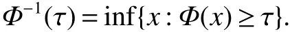
Definition 6Let ξ be an uncertain variable with regular uncertainty distribution Φ(x). Then for any real number x and 0 ≤ τ ≤ 1,the τ uncertain quantile of ξ is defined as
Definition 7For a real number τ ∈ (0,1),we define an uncertain loss function ρτ(y)as follows,

where the indicator function I{A}equals 1 for all elements of A and 0 otherwise.
According to the calculation of expectation in uncertainty theory,the expectation of uncertainty loss function in Definition 7 is proved as follows.
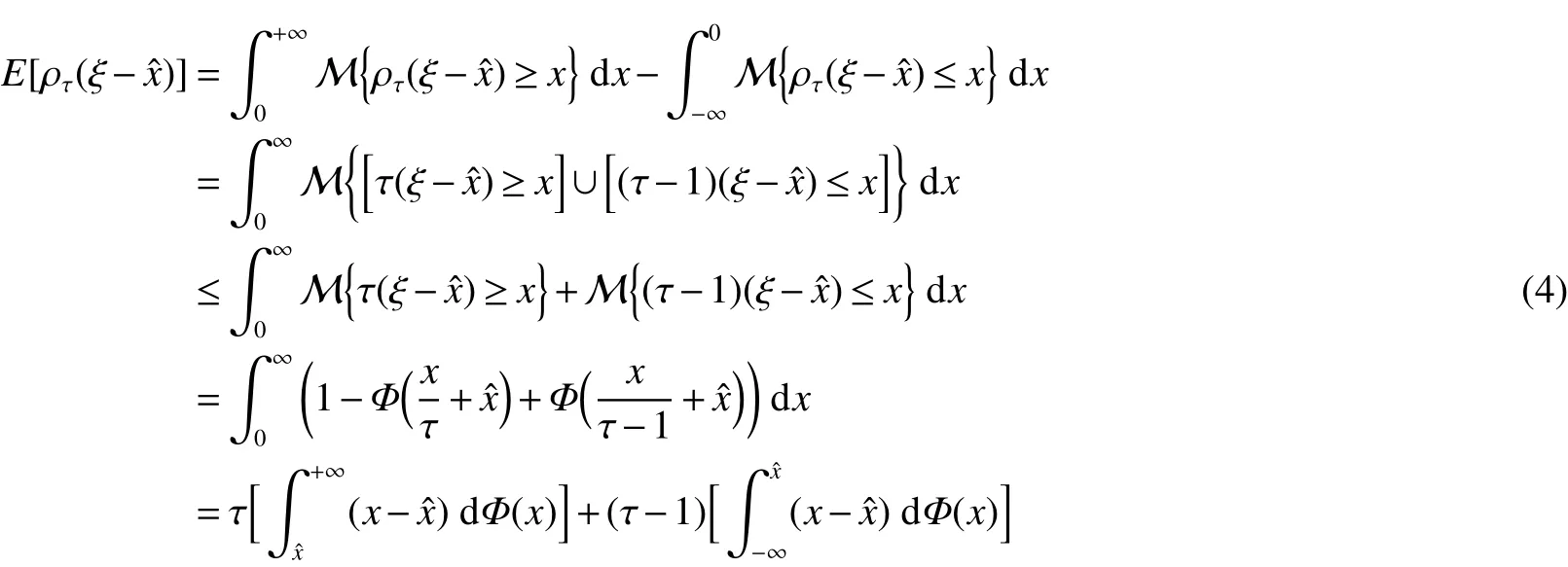
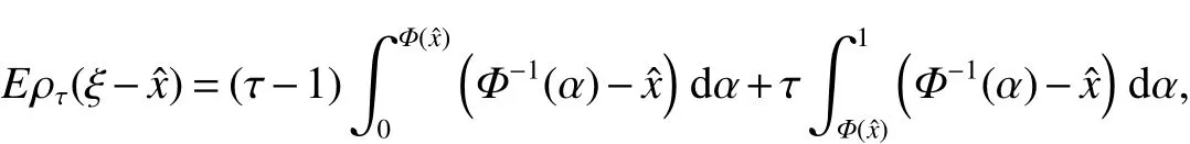
Theorem 3Let ξ be an uncertain variable with an uncertainty distribution Φ(x). If the uncertain loss function is ρτ(y),then for any real number ˆx and τ ∈(0,1),the expected value of the uncertain loss function is defined by

ProofAccording to formula(1)in Definition 7,

Denote the uncertain measure as M which reflects the personal confidence degree of an uncertain event that may happen,an uncertain variable as ξ and its uncertainty distribution as Φ(x). Then it follows from the definition of expected value[10]and subadditivity of uncertain measure[10]that
Note that ξ is uncertain variable and

is increasing with respect to ξ. The inverse distribution of the uncertain variable ξ is Φ−1(α). According to the operation law of the uncertain variable[10],and the inverse uncertainty distribution of uncertain variable(5)is
therefore,

Since Equation(4)can be showed as
for any τ ∈ (0,1).
According to uncertainty theory,the uncertain quantile can be defined as Theorem 4.
Theorem 4Let ξ be an uncertain variable with uncertainty distribution Φ(x). Then for any real number ˆx,we have
ProofAccording to the uncertain loss function ρτ(y),τ ∈ (0,1),Formula(2)and Theorem 3,we find the minimum value of the objective function:

Taking the derivative of ˆx in the Equation(2),we get

which can be calculated as

Since Φ(x)is a regular uncertainty distribution, it has a unique solution, Φ(ˆx)=τ. Therefore, the minimum estimated expectation of the real number ˆx is the uncertain quantile.
3 UQR Model
In this section,UQR model is presented,parameters are estimated for different quantiles,and the residual distributions,forecast values,confidence intervals for the corresponding quantiles are given.
3.1 Statistical Inference of UQR
The uncertain least absolute deviation estimator was derived by Liu and Yang[19].According to the definition of uncertain quantile,the uncertain quantile is 0.5 in Reference[19],while other quartiles are not explained. However,Liu and Yang only analyzed the change pattern of the data in the center,other data are not analyzed. To make up for this deficiency,we define a unary uncertain quantile regression model as follows.
Definition 8Given imprecisely observed data yi, xi(i=1,2,···,n) characterized as independent uncertain variables with regular uncertainty distributions Φi,Ψi(i=1,2,···,n). These data satisfy the unary linear regression model,i.e.,

When τ is uncertain quantile,the unary linear regression model is expressed as

where β0τ,β1τare unknown parameters,εiτare disturbance terms.
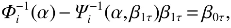
Definition 9If the data satisfy the linear regression model(6)in which τ is uncertain quantile,then uncertain quantile regression estimators β∗0τ,β∗1τof β0τ,β1τrespectively are the optimal solutions of the following minimization problem:

further,

where i=1,2,···,n,τ ∈ (0,1).
To analyze the parameter estimation problem, the parameter estimation of the UQR model can be turned to a simple optimization solution problem.
Theorem 5If the data satisfy the linear regression model(6)in which τ is uncertain quantile,then uncertain quantile regression estimators β∗0τ,β∗1τof β0τ,β1τrespectively are the optimal solutions of the following minimization problem:

further,

which can be calculated as

where

and

for i=1,2,···,n,τ ∈ (0,1).
ProofAccording to Definition 9,then UQR estimators β∗0τ,β∗1τof β0τ,β1τrespectively are the optimal solutions of the following minimization problem:

Noting imprecise observations yi, xi(i = 1,2,···,n) have uncertainty distributions Φi, Ψi(i = 1,2,···,n), so the inverse uncertainty distributions of yi, xi(i=1,2,···,n)are Φ−1i(α),Ψ−1i(α)(i=1,2,···,n). The uncertain variables

increase with the increase of yi, increase with the increase of xiwhen β1τ< 0; and increase with the decrease of xiwhen β1τ≥ 0,i=1,2,···,n,τ ∈ (0,1). According to the operation law of uncertain variables[10],the inverse uncertainty distributions of uncertain variables(9)are

where
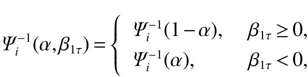
for i=1,2,···,n,τ ∈ (0,1). Therefore,we take Φ−i1(α)−β0τ−Ψi−1(α,β1τ)β1τ=0,for i=1,2,···,n,τ ∈ (0,1). Suppose Φi(α),Ψi(α)are linear uncertainty distributions,Φi(α)have inverse uncertainty distributions Φ−i1(α)=(1−α)a1i+αb1i,Ψi(α)have inverse uncertainty distributions Ψi−1(α)=(1−α)a2i+αb2i,when β1τ<0,

and

then

so that

for i=1,2,···,n,τ ∈ (0,1). When β1τ≥0,Ψi−1(1− α,β1τ)= Ψi−1(1−α)= αa2i+(1− α)b2i,
then

so that

for i=1,2,···,n,τ ∈ (0,1). According to Theorem 3,Formula(8)can be calculated as follows

where

and
for i=1,2,···,n,τ ∈ (0,1).
3.2 Stability Testing
Normally,the establishment of the statistic models should include stability testing. However,the data are imprecise in some cases, and it is difficult to test imprecise data in probility theory. So we give Definition 10 to introduce the specific method of UQR model testing using imprecise data.
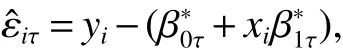
Definition 10If the data satisfy the linear regression model (6) in which τ is uncertain quantile, the residuals of τ uncertain quantile regression are expressed as

β∗0τ,β∗1τare UQR estimators of β0τ,β1τ,respectively. Furthermore,with the assumption that E[εˆiτ]=eτ,V[εˆiτ]=σ2τ,uncertain mean square errors of εiτare mseτ,(i=1,···,n),τ ∈ (0,1). We can estimate expected values,variances,mean square errors of τ uncertain quantile regression as eˆτ, σˆ2τ,mseτ,respectively.

where i=1,2,···,n,τ ∈ (0,1).
For convenience of calculation,the following formula is given based on uncertainty theory and the concept of Definition 10.
Theorem 6If the data satisfy the linear regression model(6)in which τ is uncertain quantile,then the expected values eˆτ,variances σˆ2τand uncertain mean square errors mseτof εiτcan be respectively calculated as follows

where

for i=1,2,···,n,τ ∈ (0,1)and β∗0τ,β∗1τare UQR estimators of β0τ,β1τ,respectively.
ProofAccording to Definition 10,the residuals of τ UQR are expressed as
for i=1,···,n, τ ∈ (0,1) and the valuation of β0τ, β1τare β∗0τ, β∗1τ, respectively. According to the operation law of uncertain variables[10],inverse uncertainty distributions Fi−τ1(x)of εˆiτare

where i=1,···,n,τ ∈ (0,1). Then we have
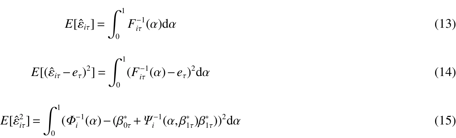
where

for i=1,···,n,τ ∈ (0,1). Theorem 6 can be directly obtained from formulas(13)∼(15).
In the following paragraphs,Definition 11 and Definition 12 give the calculations of the forecast values and confidence intervals.
Definition 11Given a new uncertain variable ˜x with a regular uncertainty distribution ˜Ψ in τ uncertain quantile regression model(6),the forecast values ˆyτare predicted to be

Definition 12Suppose in τ uncertain quantile regression, ˆετare normal uncertain variables,N(ˆeτ,ˆστ),τ ∈(0,1).Using the linear regression model(6),the uncertainty distributions of ˆyτare Φτ,and the inverse uncertainty distributions Φ−1τ(α)of ˆyτare given as follows

where

and

for τ ∈ (0,1). Θ−τ1(α)are the inverse uncertainty distributions of the normal uncertain variables N(eˆτ,σˆτ),τ ∈(0,1). Therefore,according to the subadditivity of uncertain measures[10],we have

where τ ∈(0,1). Thus,the prediction intervals of ˜x corresponding to yτare

and βτare the minimum values of Formula(16):

where τ ∈ (0,1).
4 Numerical Simulation and Case Analysis
In this section,two experiments based on Model(6)are performed. Furthermore,we estimate the unknown parameters,expected values,variances,mean square errors,forecast values and confidence intervals for the UQR model. We have a linear uncertain variable L(a,b)with the distribution

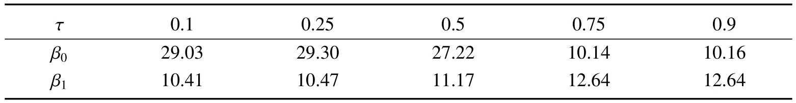
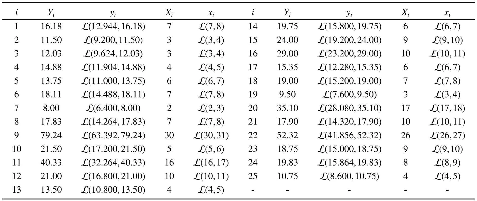
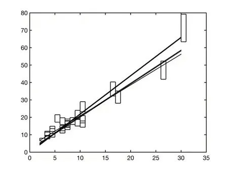
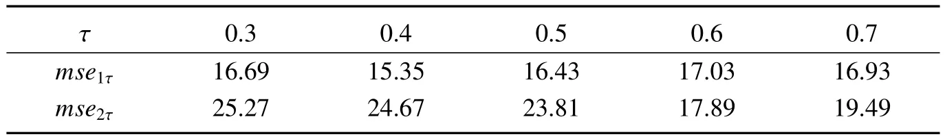
where a and b are real numbers,and satisfying a We describe the imprecise data expressed in interval forms as linear uncertain variables(Table 1). Table 1 Imprecisely observed data By Theorem 5,if the data satisfy the linear regression model(6),the unknown parameters β∗0τ,β∗1τrespectively are the optimal solutions to the following minimization problem: where and for i=1,···,n,τ ∈ (0,1). Through the formulations above,we can obtain estimates of the UQR in Table 2 when τ is equal to 0.1,0.25,0.5,0.75 and 0.9,respectively. Table 2 Estimated coefficients of each quantile According to Theorem 6,the estimated expected values and variances of ετ,τ =0.1,0.25,0.5,0.75,0.9,respectively are shown in Table 3. Table 3 Estimated expected values and variances From Table 4,it can be seen that mean square errors with imprecise observations are as follows. Table 4 Mean square errors under imprecise observations The mean square error in the UQR model can reflect the fit of different quartiles,and the whole pattern of the data can be judged based on it. As shown in Table 4, by calculating the mseτvalues at different quartiles, with the exception of the quantile with τ=0.5, all other mseτare about 300, from 0.1 to 0.5, the values of the quantiles increase and mseτdecrease.From 0.5 to 0.9, mseτincrease with the increase of quantiles. In other words, the data are mostly concentrated around the τ=0.5 quantile regression line. Next,a new imprecise observation ˜x=L(30,31)is given. From Table 5,the forecast values of the uncertain variables and the prediction intervals at the confidence level α=95%are predicted. From the values of the coefficients for each quantile in Table 2,the corresponding lines are drawn as follows(Fig 1). Table 5 Forecast values and confidence intervals Fig 1 UQR diagram of imprecise data at five quantiles The following case is taken from Reference[19]. Suppose an industrial engineer,employed by a company responsible for bottled soft drinks,is analyzing the working performance of a vending machine. A man randomly visits 25 retail stores equipped with vending machines to observe the delivery time(in minutes)and the quantity delivered(in cases)for each store in turn. Due to the data recording mechanism,imprecision of the data is inevitable,so it is more reasonable to describe imprecise data as uncertain variables. In Table 6,data Yiand Xiare from the original data in Reference[19],i=1,2,···,n,respectively.The lower limit of each uncertain data yiis the corresponding Yisubtracted from itself by 20%,and the upper limit is Yiitself,i=1,2,···,n,respectively. The lower limit of each uncertain data xiis the corresponding Xiitself,and the upper limit is the corresponding Xiof itself plus 1,i=1,2,···,n,respectively. Table 6 Data of delivery time and delivery volumes We choose a unary linear regression model to fit the uncertain observations in Table 6. According to Theorem 5,UQR estimators β∗0τ,β∗1τof β0τ,β1τrespectively are the optimal solutions of the following formula minimization problem: where for i=1,···,n,τ ∈ (0,1). Through the formulations above, we can obtain estimates of the UQR in Table 7, when τ is equal to 0.1, 0.25, 0.5,0.75, 0.9, respectively. According to Theorem 6, the estimated expected values and variances of ετ, τ=0.3,0.4,0.5,0.6,0.7,respectively are shown in Table 8. Table 7 Estimated coefficients of each quantile Table 8 Estimated expected values and variances Next,a new imprecise observation ˜x=L(31,32)is given. From Table 9,the forecast values of the uncertain variables and the confidence intervals with the confidence level α=95%are predicted. Table 9 Forecast values and confidence intervals By Table 7,the corresponding lines are drawn as follows(Fig 2). Fig 2 UQR diagram of imprecise data in different quantiles The mean square errors are mse2τin Reference[19],and the mean square errors of UQR are mse1τ. The results are as follows in Table 10. Table 10 Mean square errors In the UQR model, the mean square error is an important evaluation index. By comparing the mean square errors in Table 10, they show that the mean square errors of UQR are smaller than the mean square errors of the traditional quantile regression model in different quantiles. In other words,UQR estimation is more suitable. This paper proposes a new uncertain quantile regression (UQR) model to compensate the uncertain least absolute deviations for uncertain multivariate regression model in Reference[19]. In terms of model applications,the UQR model can reasonably describe the variation of the response variables and predictor variables at each quantile. And potential different solutions have very useful interpretative significance in different quantiles. In terms of data,uncertain data can be applied to the UQR model. This new model combines leverages uncertainty theory and quantile regression to provide a more comprehensive explanation of the problem. So the UQR model is more reasonable and reliable.4.1 Numerical Example


4.2 The Case Analysis


5 Conclusion
猜你喜欢
科技进步与对策(2022年19期)2022-10-08 12:40:34
数学年刊A辑(中文版)(2021年4期)2021-02-12 01:20:44
校园英语·月末(2020年2期)2020-05-19 15:05:49
新疆农垦科技(2016年10期)2016-06-15 20:29:33
新疆大学学报(哲学社会科学版)(2015年4期)2015-10-12 01:17:34
航天返回与遥感(2014年4期)2014-07-31 17:47:33
河南科技(2014年11期)2014-02-27 14:10:20
河南科技(2014年11期)2014-02-27 14:09:41
河北工程大学学报(自然科学版)(2014年3期)2014-02-27 13:46:20
城市道桥与防洪(2013年8期)2013-03-11 15:18:05