Research and application of stochastic resonance in quad-stable potential system

Li-Fang He(贺利芳)， Qiu-Ling Liu(刘秋玲)， and Tian-Qi Zhang(张天骐)

School of Communication and Information Engineering，Chongqing University of Posts and Telecommunications(CQUPT)，Chongqing 400065，China

Keywords: bearing fault detection，QSR，weak signal detection，SAF，W

1. Introduction

In recent decades，Stochastic Resonance(SR)[1]has been widely studied in physics，[2–4]biology，[5–7]and many other scientific fields.[8–12]SR is a phenomenon showing the fluctuation force acts on the system non-linearly.[13–15]The SR theory was first introduced by Benziet al.[13]in the 1990s while exploring the glacial period. Subsequently， more novel SR theories have emerged. McNamaraet al.[16，17]proposed adiabatic approximation theory based on transition probability. Due to the limitations of small parameters in the adiabatic approximation theory， Dykmanet al.[18]proposed the linear response theory to characterize SR more comprehensively. Then， Junget al.[19–21]analyzed the SNR through the Fokker–Planck equation(FPE).

Currently，some of the famous potential function models have emerged from researchers worldwide， including: classical bistable SR，[22–25]exponential bistable SR，[26]coupled bistable SR，[27–29]and other tri-stable and multi-stable potential function models. Tan Chunlinet al.[30]presented the application of standard tri-stable SR system in early bearing fault diagnosis. Yang Yuleiet al.[31]proposed the research on a self-adaptive， cascaded tri-stable SR system under Levy noise. Zhang Buet al.[32]proposed the tri-stable state system powered by additive and multiplicative noise，and studied its mean first passage time(MFPT)and steady-state probability density(SPD).Liet al.[33]proposed an adjustable steadystate system and concluded that there were various nonlinear potential functions in the tri-stable system. Subsequently， researchers have successively studied the compound tri-stable potential function，[34]etc. In addition， there are also lots of novel SR，such as fractional SR，[35，36]stable-matching SR[37]and even SR-based signal decomposition.[38]There have been extensive researchers performed on the application of SR in bearing fault diagnosis. For example， Liuet al.[39]converted large frequency signals into small frequency signals through the frequency domain information exchange method.

Although researchers have studied the bistable and tristable systems from various aspects， there are still few studies on quad-stable or even multi-stable systems， which need further research. In this paper， a new Quad-stable potential stochastic resonance(QSR)is submitted. The structure in this paper is as follows: In Section 2，a system model is proposed and compared with CTSR. Additionally， the expressions of SPD， MFPT，W， and SAF are derived. In Section 3， QSR is compared with CTSR through numerical simulation under low-frequency， high-frequency， and multi-frequency signal conditions. And the variation of SNR and MSNRI is investigated with noise intensityDfor two systems. In Section 4， 6205-2RS JEM SKF and HRB 6205-2Z models are chosen for bearing fault detection. Finally，the conclusions of this paper are presented in Section 5.

2. QSR analysis

2.1. Introductions on QSR

Under the over-damping condition， the dynamic Langevin equation of SR can be obtained:

where，ζ(t) is the Gaussian white noise with〈ζ(t)〉= 0，〈ζ(t)ζ(t-t′)〉=2Dδ(t′)， andU(x，t)is the quad-stable generalized potential function andU0(x) is the system potential function as follows:

ε(t)=Asin(2π ft+φi)is the input periodic signal where the phase is usually ignored which can be simplified asε(t) =Asin(2π ft).U0(x)can be expressed by parametermas shown in Eq.(3):

where

U0(x)has four steady-state points:

Figures 1(a) and 1(b) are the potential function ofU0(x)andU1(x)，respectively. By adjustingm，it can be found that it is a quad-stable state when 0＜m ≤2，a tri-stable state when 2＜m ≤4 and a bistable state when 4＜m ≤6.

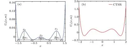
Fig.1. Potential functions of U0(x，m)and U1(x): (a)U0(x，m)of QSR(m=1.5)，(b)U1(x)of CTSR(a=1.5，b=3，and c=1).

Figure 2 is the potential function of QSR withm. It can be seen that the potential well ofU0(x，m)on both sides shifts to the right and the well depth changes asmincreases， while the middle potential well changes insignificantly.

Figure 3(a)shows the variation of the potential well force，which is symmetric about the origin and fluctuates between(-0.5， 0.5). It can be concluded that the nonlinear forces play an essential role on the shape of potential force. Figure 3(b)shows the height of the potential barriers. Whenmis less thanmc，all barriers’height is increasing，and the middle one is higher than the others， which indicates that the particles need more energy to transit from the middle wells to the outer wells. In contrast whenmis higher or equal thanmc，the particle needs less energy. The height of the middle barrier is Δu0=m4(m2-8m+12)2/2048，and Δu1=Δu2=m4/128 for the other barriers.

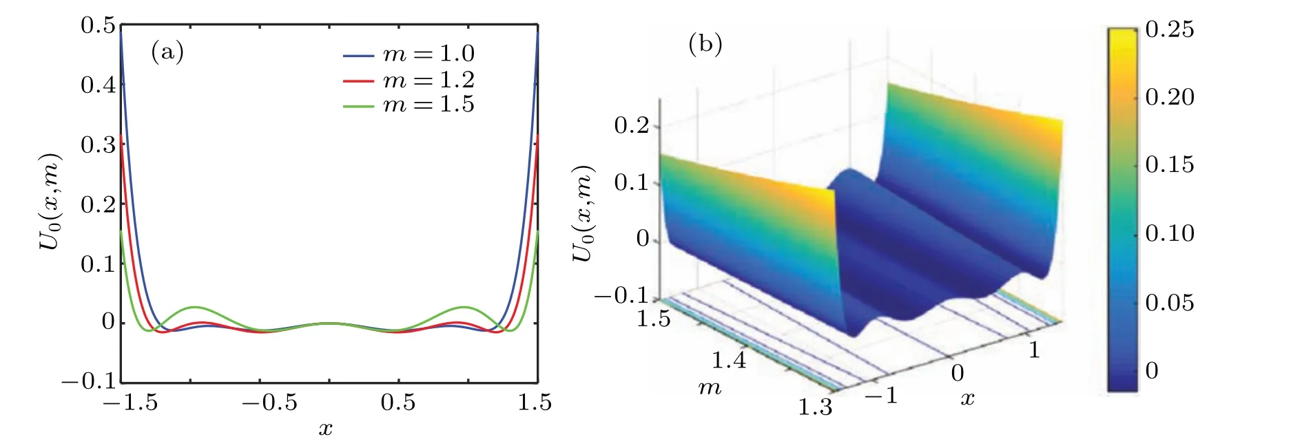
Fig.2.U0(x，m)varies with m and x: (a)U0(x，m)varies with m and x，(b)U0(x，m)varies with m and x.

Fig.3. Potential well force and potential barrier: (a)potential well force，(b)potential barrier.

2.2. SPD of QSR

From Eq.(1)，the corresponding FPE is:

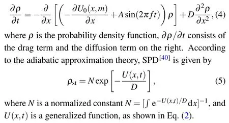
SettingA=0，figure 4 shows the impacts ofmandDon SPD.Studying the relationship betweenρstand each parameter facilitates the analysis of the particle motion state. Therefore，by keepingmfixed and increasingD，the overall trend in the potential wells on both sides and the middle potential well remains unchanged. But the peak value is smaller， indicating that the particle transition requires less energy.WhenDis constant，the depth of the outer potential wells getting deeper and that of the inner well is shallower asmincreases， indicating that the particles are easier to transit from the inner potential wells to the outer wells.

Fig.4. ρst varies with D，m，and x: (a)ρst varies with D and x(m=0.95)，(b)ρst varies with D and x(m=0.95)，(c)ρst varies with m and x(D=0.2)，(d)ρst varies with m and x(D=0.2).

2.3. MFPT of QSR

Figures 5–7 show changes of MFPT withmandD. FixingDand increasingm， whenm ＜1，T12increases with increasingD，whenm ≥1，T12decreases with increasingD. The smallerT12， the greater the probability of particle transition，which indicates easier particle transition and stronger SR characteristics.T43shows the same characteristics asT12. In the same way，T34andT23both decrease monotonously with the increase ofDand the escape rate of particles increases. FixingDand increasingm，T34andT23decrease.T21has the same characteristics asT34，T32has the same characteristics asT23.The above results show that the escape rate of the particle is greater asmandDincrease，which indicates stronger SR characteristics.

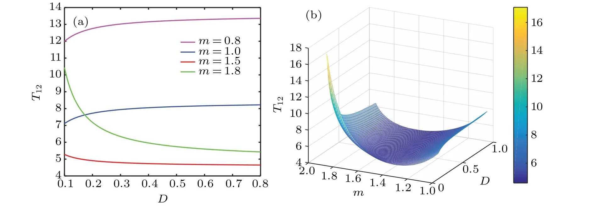
Fig.5. T12 or T43 varies with D and m: (a)T12 or T43 varies with D and m，(b)T12 or T43 varies with D and m.

Fig.6. T34 or T21 varies with D and m: (a)T34 or T21 varies with D and m，(b)T34 or T21 varies with D and m.

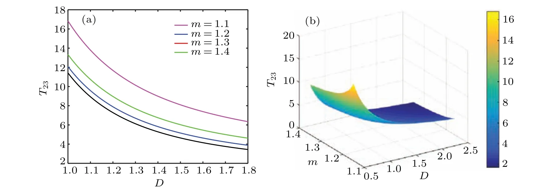
Fig.7. T23 or T32 varies with D and m: (a)T23 or T32 varies with D and m，(b)T23 or T32 varies with D and m.

2.4. WWW of QSR

Eq.(10)，it can be shown as[41]

Then，P=(P1，P2，P3，P4)can be obtained as:

When there is an external force，the expression of its potential function isU(x，t)=U0(x)-xε(t)，then differentiation obtains the expression:

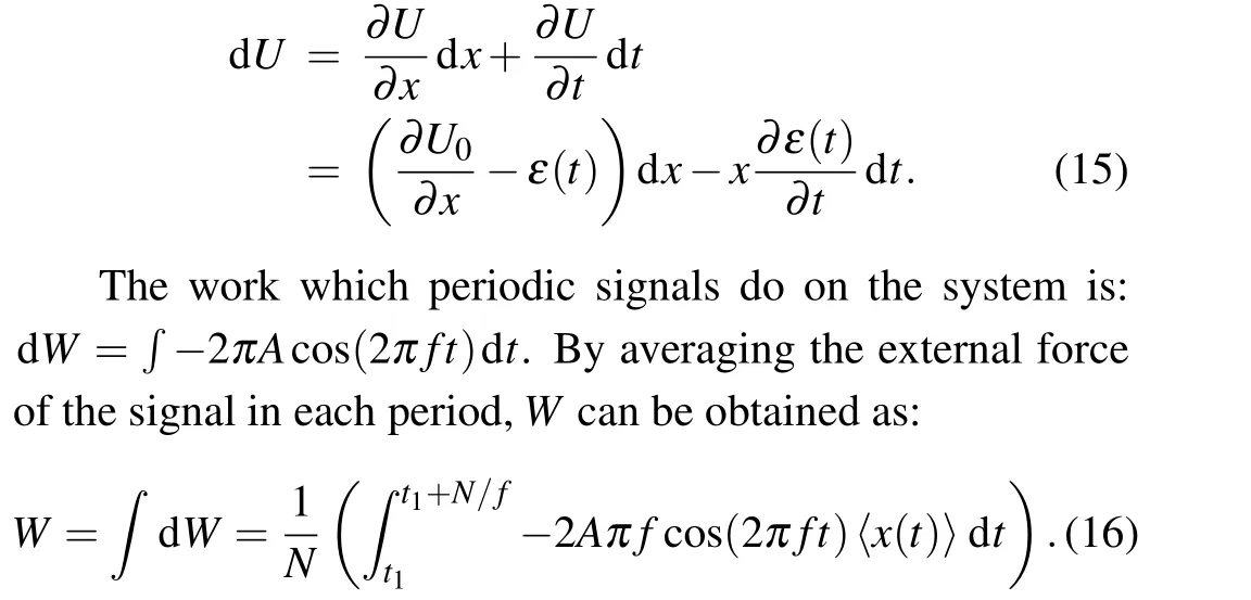
Figure 8 shows the relationship between〈x(t)〉andD.WhenA=0.0025，f=0.001，N=300，〈x(t)〉varies periodically withD，indicating that the particles vibrate with largerDand the transition time.

Figure 9 shows the change ofWwithDandm，Wfirst increases and then decreases asDincreases. By fixingDand increasingm，Wshows a single peak. By adjustingm， the single peak can be converted to the double peak，but the peak value is reduced. This is because the QSR have the double quad-stable’s characteristics when 0＜m ≤2，which is consistent with the theory.

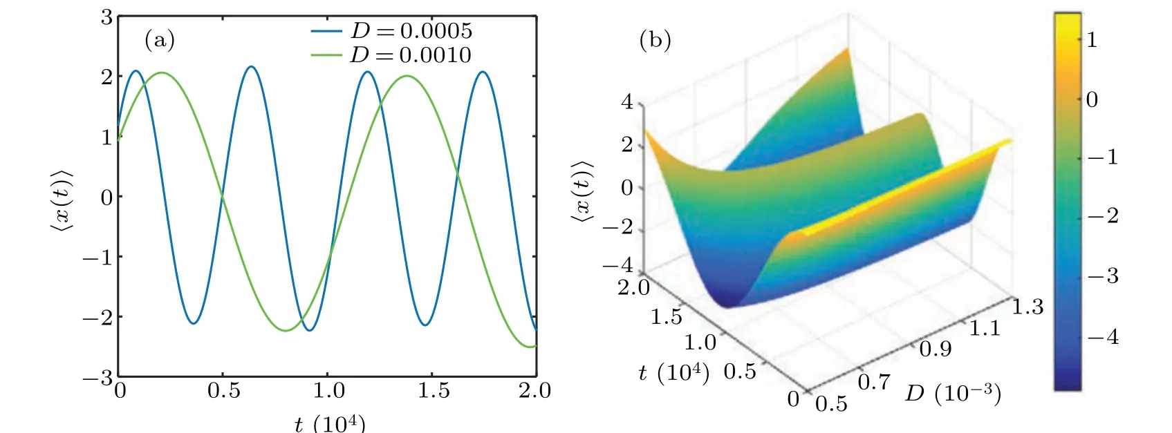
Fig.8. 〈x(t)〉varies with D and t: (a)〈x(t)〉varies with D and t (m=0.6)，(b)〈x(t)〉varies with D and t (m=0.6).

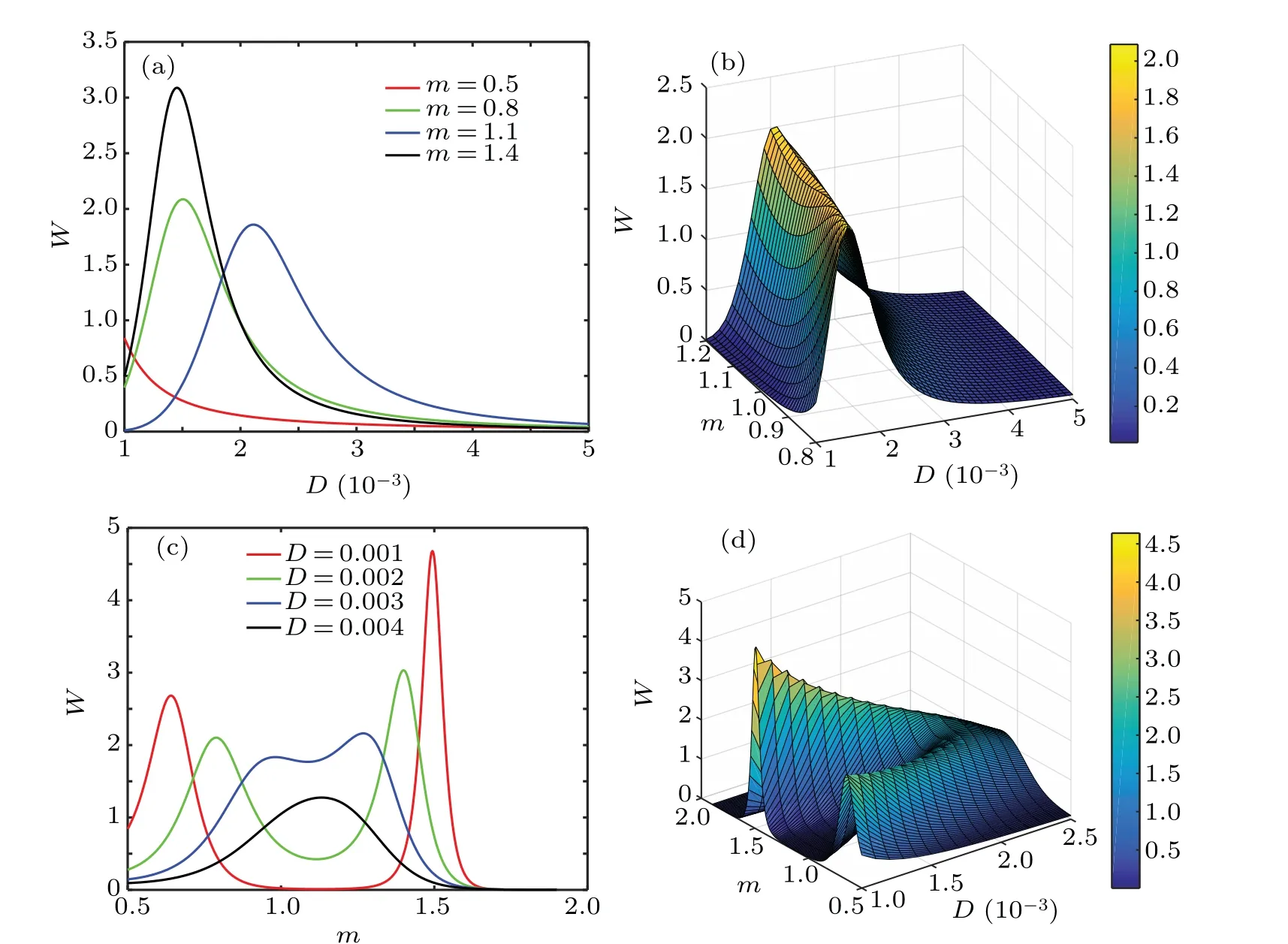
Fig.9.W varies with D and m: (a)W varies with m，(b)single peak，(c)W varies with D，(d)double peak.

2.5. SAF of QSR

By simplifying the conditional probability and Eq.(13)

Under the limitation of a long time，the output power of〈x(t)〉2is

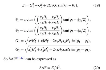
Fig.10. Variation of SAF with A，m， f: (a)SAF varies with D and A(m=1.5)，(b)SAF varies with D and A(m=1.5)，(c)SAF varies with D and m，(d)SAF varies with D and m，(e)SAF varies with D and f (m=1.2)，(f)SAF varies with D and f (m=1.2).

Figure 10 shows the effects ofA，m， andfon SAF， it can be seen that SAF increases first and then decreases. In Fig.10(a)and Fig.10(b)，when other parameters remain fixed，SAF is proportional toAandmand the peak increases with the increase ofAandm，respectively. In Fig.10(c)，SAF is steeper than that in Fig. 10(a)， indicating thatmis more sensitive to SAF thanA. In Fig.10(e)and Fig.10(f)，fhas little effect on the peak of SAF，which is inversely proportional tof，and the peak shifts to right whereDis bigger asfincrease.

3. Numerical simulation and engineering application

To verify the rules of the above theoretical analysis， GA and the fourth-order Runge–Kutta algorithm are combined to perform numerical simulations to obtain the optimal parameters:m=0.956，a=1.5125，b=3.0301，c=1.0185. In Fig.11，the noise signal is processed by QSR with a stronger periodicity and a higher amplitude， which is about 40 times than CTSR at low frequency conditions(f=0.1Hz). The frequency band of the noise is also shifted by QSR.

In Fig.12，the original signal’s spectral amplitude is 75.49 before any processing. Then it is processed by QSR to obtain more periodicity and greater amplitude which is 539.7 and is 4 times that of CTSR and 7 times that of the original signal at high frequency conditions(f=25 Hz). The results show that the amplification performance of QSR is higher than CTSR in low frequency and high frequency conditions.

Figures 11 and 12 show the time domain and frequency domain figures of the low and the high-frequency signal， setting the frequency of the periodic signal to 0.01 Hz and 25 Hz respectively. To verify that QSR has superior amplitude amplification and periodicity than CTSR not only at low frequencies and at high frequencies， but also at multi-frequencies.Then the periodic signal is added:ε(t)=0.1sin(2π×0.05t)+0.3sin(2π×0.03t)+0.5sin(2π×0.01t). Obviously， from Fig.13 the amplitude are 2.6 times， 1.1 times and 1.83 times that of the original multi-frequency signal amplitude， respectively， at 0.01 Hz， 0.03 Hz， and 0.05 Hz after CTSR processing. The amplitude are 6.9 times， 2.08 times， and 3.27 times that of the original multi-frequency signal amplitude after QSR processing. It can be seen that the amplification capability is stronger and the periodicity is better after QSR under high frequency and multi-frequency.

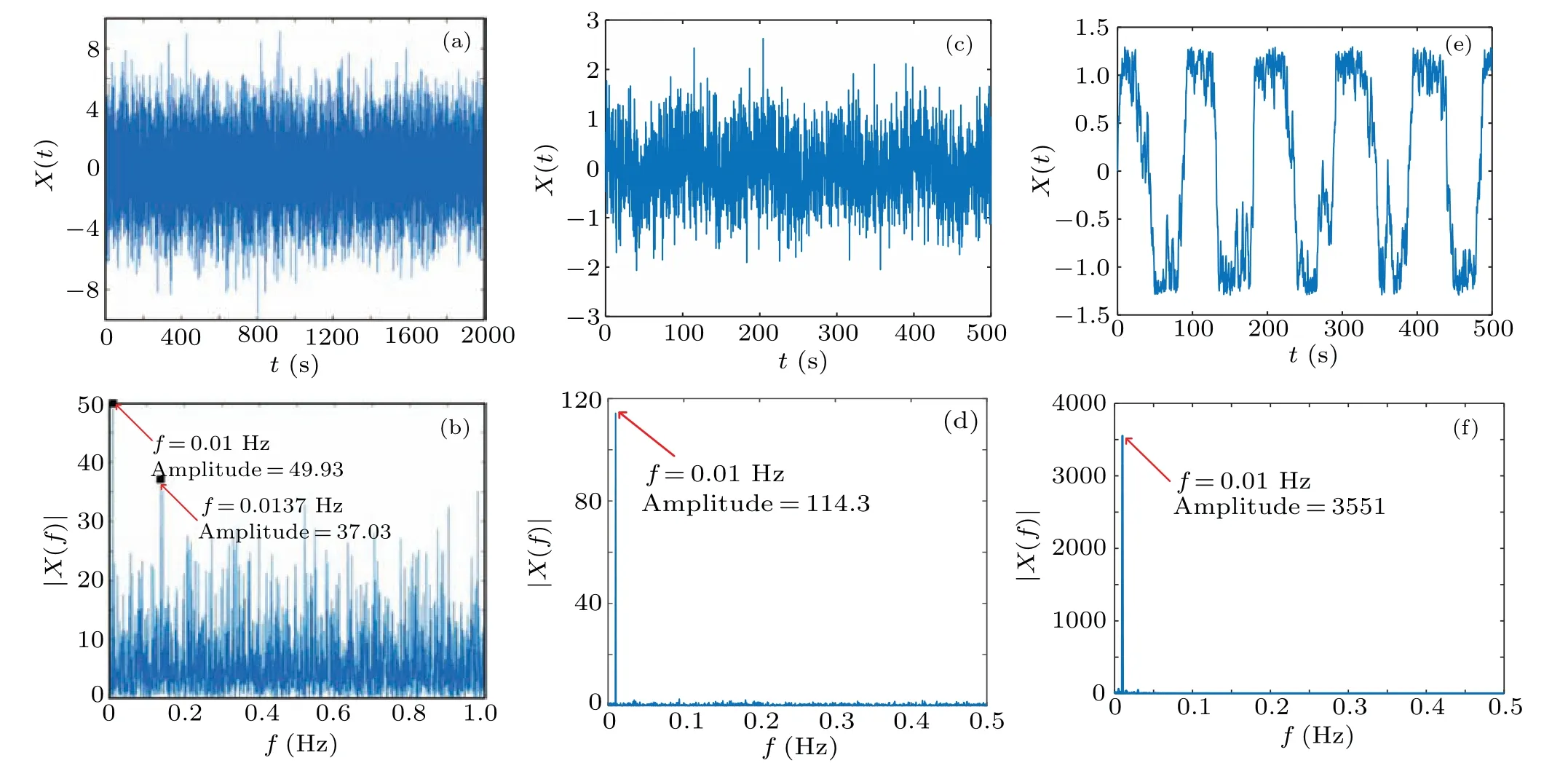
Fig.11. Compare the time and frequency domains of two systems at low frequencies(0.01 Hz): (a)time domain diagram of input noise，(b)frequency domain diagram of input signal， (c) time-domain diagram with noise of CTSR， (d) frequency domain diagram with noise of CTSR， (e) time-domain diagram with noise of QSR，(f)frequency domain diagram with noise of QSR.

Fig. 12. Comparison of the time and frequency domains of two systems at high frequencies (25 Hz): (a) time domain diagram of input noise， (b)frequency domain diagram of input signal， (c) time-domain diagram with noise of CTSR， (d) frequency domain diagram with noise of CTSR， (e)time-domain diagram with noise of QSR，(f)frequency domain diagram with noise of QSR.

Fig. 13. Comparison of the time and frequency domains of two systems at multi-frequency: (a) time domain diagram of input noise， (b) frequency domain diagram of input signal， (c) time-domain diagram with noise of CTSR， (d) frequency domain diagram with noise of CTSR， (e) time-domain diagram with noise of QSR，(f)frequency domain diagram with noise of QSR.

Fig.14. Comparison of SNR and MSNRI:(a)comparison of SNR(m=0.2，a=1.8，b=3，c=1)，(b)comparison of MSNRI(m=1.5，a=1.8，b=3，c=1).

In Fig. 14， SNR of QSR is about 2 times and MSNRI is about 12 times than CTSR， where the peak of SNR in QSR and CTSR is-18.47 dB and-37.89 dB， respectively. The peak of MSNRI in QSR and CTSR is 13.93 dB and 1.144 dB，respectively， which shows that SNR of QSR is improved by 19.42 dB relative to CTSR.This indicates QSR is superior in noise immunity.

4. Bearing fault detection and application

4.1. 6205-2RS JEM SKF bearing fault detection

To verify the feasibility of QSR in practical engineering applications under different scenarios，the performance of QSR and CTSR for detecting faults is compared in this section.Due to the small public data set of actual bearing faults， the data from Case Western Reserve University (CWRU)， model 6205-2RS JEM SKF[41]is widely used by domestic and international scholars. The experimental rig is shown in Fig.15.

Fig.15. 6205-2RS JEM SKF deep groove ball bearing test device.

(i) Inner ring fault detection

Figures 16(a) and 16(b) show the time–frequency diagrams of the bearing inner ring fault signal， and the characteristic frequency of the fault signal cannot be identified. Figures 16(c)–16(f) are the time–frequency diagram of the output signals of CTSR and QSR.Due to the limitation of small parameters， secondary sampling is used for pre-processing，and the sampling frequency isfsr= 5 Hz. Then， the optimal parameters of the two systems can be obtained by GA，the optimal parameters of CTSR and QSR are:a=1.2154，b=2.5492，c=1.01596， andm=1.38641. From Fig.16(c)，Fig. 16(d)， Fig. 16(e)， and Fig. 16(f)， it can be seen that the frequency domain diagrams of the two systems show peaks atf=162 Hz(relative error is 0.123%).At this time，the SNR of QSR and CTSR are-3.7363 dB and-2.8159 dB respectively，which is an improvement of 0.9204 dB.QSR has a larger peak and less noise interference than CTSR，which makes easier to detect the inner ring fault and indicates the superiority of QSR.

Fig. 16. Inner ring fault detection of CTSR and QSR: (a) Time domain of inner ring fault signal， (b) frequency domain of inner ring fault signal， (c)inner ring fault detection time domain of CTSR，(d)inner ring fault detection frequency domain of CTSR，(e)inner ring fault detection time domain of QSR，(f)inner ring fault detection frequency domain of QSR.

(ii) Outer ring fault detection

Figures 17(a) and 17(b) show the time–frequency diagrams of the bearing outer ring fault signal. It can be seen that the fault signal is completely submerged in noise and the characteristic frequency of the fault signal cannot be identified. QSR and CTSR are used to detect the fault signal. Then，the optimal parameters of the two systems can be obtained by GA. The optimal parameters of CTSR are:a= 1.0028，b=2.16974，c=1.0095， and the optimal parameter of QSR is:m=1.09348. Comparing Fig.17(c)，Fig.17(d)，Fig.17(e)，and Fig. 17(f)， it can be seen that the frequency domain diagrams of both systems show peaks atf=108 Hz (the relative error is 0.65%)， which indicates that the characteristic frequency of the fault signal is detected. Figures 17(e) and 17(f) are the output signal of QSR， it can be seen that the time domain signal exhibits periodicity and the peak of the spectrum atf=108 Hz is nearly 2 times higher than CTSR.At this time， the SNR of QSR and CTSR is-38.4624 dB and-36.6194 dB， respectively， which is an improvement of 1.842 dB compared with CTSR.The results indicate that QSR has a better detection performance than CTSR.

Fig. 17. Outer ring fault detection of CTSR and QSR: (a) time domain of outer ring fault signal， (b) frequency domain of outer ring fault signal， (c)outer ring fault detection time domain of CTSR，(d)outer ring fault detection frequency domain of CTSR，(e)outer ring fault detection time domain of QSR，(f)outer ring fault detection frequency domain of QSR.

4.2. HRB 6205-2Z bearing fault detection

To demonstrate the availability of QSR in different scenarios，another fault data model HRB 6205-2Z is selected for fault detection. The main parameters[43]are shown in Table 1， the experimental station of HRB 6205-2Z in Fig. 18.The sampling frequency is 20 kHz， according to Eq. (21)，the inner raceway frequency and outer raceway frequency of the bearing can be obtained theoretically as 117.14 Hz and 78.13 Hz respectively. The proportional compression rate and the secondary sampling frequency areR= 4000 andfsr=fs/R=5 Hz，the calculation step ish=1/fsr=0.2.

wherenis the number of rolling elements，flis rotation frequency，dis diameter of rolling element，Dlis pitch diameter andβis bearing contact angle.

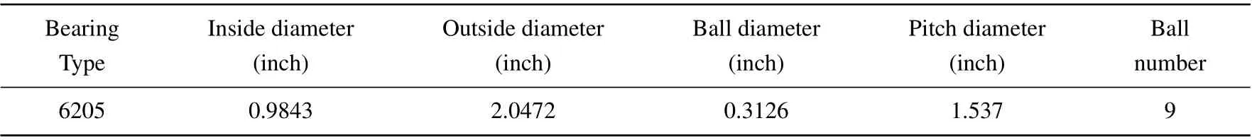
Table 1. The main structure parameters of the tested bearing HRB 6205-2Z.

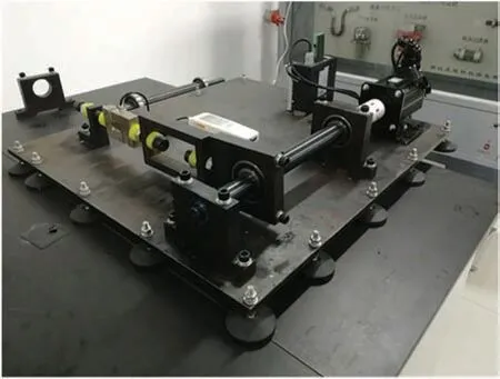
Fig.18. The experimental station of HRB 6205-2Z.

(i) Inner ring fault detection

The optimal parameters of the two systems can be obtained by GA.The optimal parameters of CTSR and QSR are:a=1.3235，b=2.9574，c=1.0028，m=1.4459.Figures 19(a)and 19(b)show the time–frequency diagrams of the fault signal. It can be seen that the signal is submerged in noise and the characteristic frequency of the fault signal cannot be identified. Figures 19(c)–19(f)are the time–frequency diagrams of the output signals of CTSR and QSR， respectively， in which shows that fault is highlighted atf= 116 Hz (the relative error is 0.973%). At this time， the SNR of QSR and CTSR is-29.9642 dB and-31.9351 dB， respectively， which is an improvement of 1.9709 dB.Furthermore，the output signal of QSR has higher spectral peaks and less noise， indicating that QSR has better anti-noise and detection performance.

Fig. 19. Inner ring fault detection CTSR and QSR: (a) time domain of inner ring fault signal， (c) inner ring fault detection time domain of CTSR， (b)frequency domain of inner ring fault signal，(d)inner ring fault detection frequency domain of CTSR，(e)inner ring fault detection time domain of QSR，(f)inner ring fault detection frequency domain of QSR.

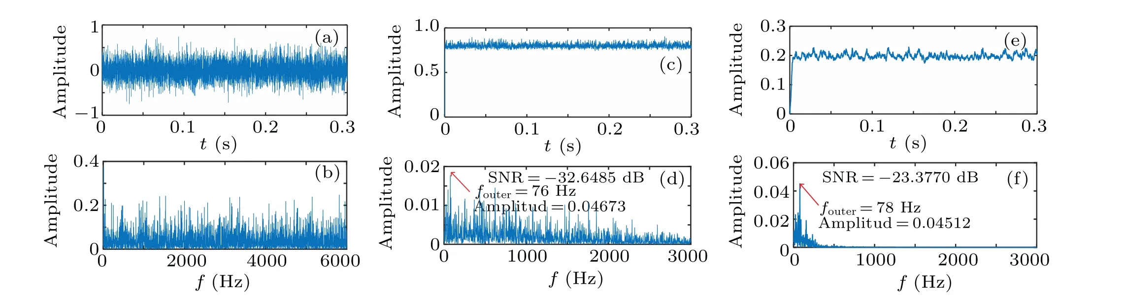
Fig.20. The outer ring fault detection of CTSR and QSR:(a)time domain of outer ring fault signal，(b)frequency domain of outer ring fault signal，(c)outer ring fault detection time domain of CTSR，(d)outer ring fault detection frequency domain of CTSR，(e)outer ring fault detection time domain of QSR，(f)outer ring fault detection frequency domain of QSR.

(ii) Outer ring fault detection

Similarly，the optimal parameters of the two systems can be obtained by GA.The optimal parameters of CTSR and QSR are:a=1.5021，b=3.0121，c=1.1129，m=1.5137. Figures 20(a) and 20(b) illustrate the time–frequency diagrams of the outer ring fault signal. It can be seen that the signal is submerged in noise and the characteristic frequency of the fault signal cannot be identified. Figures 20(c)–20(f) are the time–frequency diagrams of the output signals of CTSR and QSR.It can be seen that CTSR detected the fault atf=76 Hz(the relative error of 2.731%) and QSR detected the fault atf=78 Hz (the relative error of 0.166%). Apparently， QSR has a lower relative error in fault detection. At this time， the SNR of QSR and CTSR is-23.377 dB and-32.6485 dB，respectively which is an improvement of 9.2715 dB compared with CTSR.The output signal has a higher spectral peak and less noise，indicating that QSR has better noise immunity and detection performance than CTSR.

5. Conclusion and outlook

This paper overcomes the problem of low performance of weak signal enhancement in multi-stable systems and proposes a better QSR. Firstly， the characteristics of MFPT，W，SAF，SNR，and MSNRI are studied and used as the measurement indexes. Then， GA and fourth-order Runge–Kutta algorithm are used to compare the SNR and MSNRI of CTSR and QSR.Finally，CTSR and QSR are applied in bearing fault diagnosis. The conclusions are as follows:

(i) MFPT first increases and then decreases asmandDincrease，i.e.，the SR phenomenon occurs，andmis more sensitive to MFPT.

(ii)Walso first increases and then decreases asDincreases.Because the system has the double quad-stable’s characteristics when 0＜m ≤2，the double peak ofWoccurs.

(iii) SAF is proportional toAandm，but is inversely proportional tof. Moreover，mis more sensitive to SAF andfhas little effect on SAF.

(iv) According to simulation results，the amplification capability of QSR is superior than CTSR at low frequency(f=0.01 Hz)， high frequency (f= 25 Hz) and multi-frequency signals.

(v) According to simulation results，the SNR and MSNRI of QSR are about 2 times and 12 times higher than CTSR respectively，indicating better performance.

(vi) Under the 6205-2RS JEM SKF bearing fault detection， the amplitude of the inner and outer ring output signals of QSR is 3 times and 2 times higher than CTSR，respectively.For HRB 6205-2Z bearing fault detection，the amplitude of the inner and outer ring output signals of QSR is 13 times and 3 times higher than CTSR，respectively.And the SNR of QSR is larger than CTSR in both types of bearing fault. It shows that QSR is superior and has better noise immunity.

Future research will be focused on the theoretical analysis of the SNR and bearing fault detection under variable operating conditions.

Acknowledgements

Project supported by the National Natural Science Foundation of China (Grant No. 61771085) and the Research Project of Chongqing Educational Commission(Grant Nos.KJ1600407 and KJQN201900601).