Research on submesoscale eddy and front near the South Shetland Islands (Antarctic Peninsula) using seismic oceanography data

YANG Shun, SONG Haibin* & ZHANG Kun

Research on submesoscale eddy and front near the South Shetland Islands (Antarctic Peninsula) using seismic oceanography data

YANG Shun1,2, SONG Haibin1,2*& ZHANG Kun1,2

1School of Ocean and Earth Science, Tongji University, Shanghai 200092, China;2State Key Laboratory of Marine Geology, Tongji University, Shanghai 200092, China

The submesoscale processes, including submesoscale eddies and fronts, have a strong vertical velocity, can thus make important supplements to the nutrients in the upper ocean. Using legacy multichannel seismic data AP25 of cruise EW9101 acquired northeast of the South Shetland Islands (Antarctic Peninsula) in February 1991, we identified an oceanic submesoscale eddy with the horizontal scale of ～4 km and a steep shelf break front that has variable dip angles from 5oto 10o. The submesoscale eddy is an anticyclonic eddy, which carries warm core water, can accelerate ice shelves melting. The upwelling induced by shelf break front may play an important role in transporting nutrients to the sea surface. The seismic images with very high lateral resolution may provide a new insight to understand the submesoscale and even small-scale oceanic phenomena in the interior.

submesoscale eddy, shelf break front,seismic oceanography,South Shetland Islands

1 Introduction

Heat and material transports in oceans play a dominant role in regulating global climate and in controlling the oceanic absorption of greenhouse gases that are responsible for global warming (Zhang et al., 2014). Oceanic eddies have been recognized as key contributors in transporting heat, dissolved carbon, and other biogeochemical tracers (McGillicuddy et al., 2007; Dong et al., 2014). Surface- intensified mesoscale eddies have been studied extensively using altimetric observations (Chelton et al., 2007). However, we know much less about the contribution of subsurface eddies, particularly submesoscale ones, due to their small spatial and temporal scales (McWilliams, 2016). Same as submesoscale eddies, oceanic fronts are also submesoscale processes (Capet et al., 2008; McWilliams, 2016). The submesoscale processes, including submesoscale eddies and fronts, have a strong vertical velocity that can even reach 100 m·d−1. These submesoscale processes can sustain vertical secondary circulation with time scales comparable with the nutrient uptake by phytoplankton, thus make important supplements to the nutrients in the upper ocean (McGillicuddy et al., 2007; Zhang et al., 2019).

Oceanic eddies can be divided into cyclonic and anticyclonic eddies based on their different rotation modes. The cyclonic and anticyclonic eddies rotate counterclockwise (clockwise) and clockwise (counterclockwise) in the northern (southern) hemisphere, respectively (Pingree and Le Cann, 1992). There are downwellings in anticyclonic eddies for the Coriolis force induced by the earth’s rotation, thus can form concave isopycnal/isothermal surfaces (Zhang et al., 2014).

Different from oceanic eddies and fronts in the low and middle latitudes, those in polar regions are more important in regulating global climate for a large number of ice shelves in polar regions. A study by NASA found that ocean waters melting the undersides of Antarctic ice shelves are responsible for most of the continent’s ice shelf mass loss (Rignot et al., 2013). The eddies can carry warm-core water mass for a long distance, while almost maintaining the properties of core water. Thus, the core water mass that is warmer than surface waters will melt the undersides of Antarctic ice shelves (Gunn et al., 2018). Up to now, however, there are few researches on imaging water columns using seismic data in polar regions except Gunn et al. (2018).

Here, we found a submesoscale eddy and a shelf break front in north of the South Shetland Islands (SSI) using a new method named seismic oceanography (SO). SO uses multichannel seismic (MCS) reflection data to produce detailed images of the water column (Holbrook et al., 2003; Holbrook and Fer, 2005; Ruddick et al., 2009). Seismic imaging (i.e., acoustic reflection) can be approximately thought to be the smoothed vertical gradient of seawater temperature (Ruddick et al., 2009). Compared with the traditional physical oceanography methods, SO has the advantages of high acquisition efficiency, very high lateral resolution (～10 m) and full depth imaging of seawater column (Dong et al., 2010; Song et al., 2021). Many researchers have used seismic data to image oceanic eddies in different regions, including the west exit of the Mediterranean Sea (Biescas et al., 2008; Pinheiro et al., 2010; Song et al., 2011), South China Sea (Huang et al., 2013), Gulf of Alaska (Tang et al., 2014, 2020), southeast of New Zealand (Gorman et al., 2018), Bellingshausen Sea (Gunn et al., 2018), Middle Atlantic Bight (Gula et al., 2019), Southwest Atlantic Ocean (Gunn et al., 2020), Northwest Pacific Ocean (Zhang et al., 2021) and the Pacific coast of Central America (Yang et al., 2021). Compared with eddies, the researches on oceanic fronts are less and mainly consist of Newfoundland Basin of Northwest Atlantic Ocean (Holbrook et al., 2003), east of Japan (Nakamura et al., 2006), and Southwest Atlantic Ocean (Gunn et al., 2020). They used seismic data, combined withstation observations such as Conductivity-Temperature-Depth (CTD) and eXpendable Bathy-Thermograph (XBT), remote sensing observations of sea surface temperature (SST), sea surface height (SSH), chl-concentration, and sometimes numerical simulations of fluid dynamics, to study the oceanic eddies and fronts.

Figure 1 Bathymetry of the study region. The red line is seismic line AP25, and the 5 red dots are CTD stations in February. The isolines are isobaths of 100, 200, 500, 1000, 2000, 3000, 4000, and 5000 m, respectively. SSI = South Shetland Islands and EI = Elephant Island.

2 Oceanographic setting

SSI is located in southern Drake Strait and the northern tip of the Antarctic Peninsula (AP). Due to the complex topography, the water masses and circulations around the SSI are complex and variable (Zhou et al., 2006). The dominant circulations north of the SSI are the northeastward Antarctic Circumpolar Current (ACC) and Antarctic Slope Current (ASC) that flow southwestward along the outer shelf. As the only eastward circulation connecting the major oceans, ACC consists of a series of oceanic fronts. From north to south, these fronts are Subantarctic Front (SF), Polar Front (PF), Southern ACC Front (SACCF), and Southern Boundary (SB) (Orsi et al., 1995; Zhou and Zhu, 2020).

The waters associated with the ACC are the warm Antarctic Surface Water (ASW), the cold Winter Water (WW) below the ASW, and the warm Circumpolar Deep Water (CDW). The CDW can be further separated into the Upper CDW (UCDW) and the Lower CDW (LCDW) based on their origins from the Indian-Pacific oceans and the Atlantic Ocean, respectively (Zhou et al., 2010). WW is caused by the salt precipitation of sea ice, the sensible heat dissipation to the atmosphere, and the vertical mixing of seawater driven by wind (Zhou and Zhu, 2020). Figure 2 shows the properties of these water masses surrounding SSI.

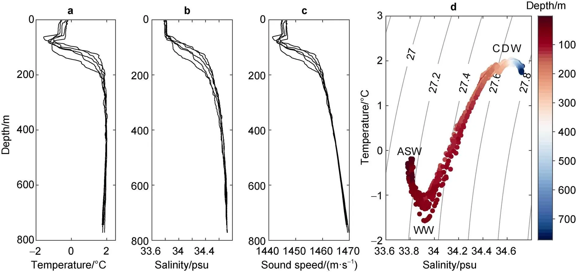
Figure 2 The legacy CTD data. a,Temperature; b,Salinity; c,Sound speed profiles; d,diagram. ASW = Antarctic Surface Water, WW = Winter Water, and CDW = Circumpolar Deep Water. The color of the dots indicates the depth of the samples. The contours are corresponding density anomalies calculated by the equation of the state of seawater.

3 Seismic data and hydrographic data

3.1 Seismic acquisition and processing

Multi-channel seismic data was acquired during R/V Maurice Ewing Expedition EW9101 conducted in February 1991. The original purpose of the seismic data acquisition is the geophysical study of the Pacific margin of Antarctica, including the Antarctic Peninsula and areas south to the intersection of the Heezen Fracture Zone with the margin. The acoustic source is an airgun array with a capacity of 136.9 L (8353 cu in). The shot interval was 20 s for ～50 m, and the nominal distance between the shot and the nearest channel is 263 m. There are 144 channels originally recorded, and group spacing is 25 m. The sample interval is 4 ms, and the record length is 12 s. Here we only use seismic line AP25 that acquired on 22 February 1991, to analyze the water masses. Note that there are only 120 channels available because the nearest 24 channels are empty and no data is recorded, hence the actual distance between the shot and the nearest effective channel is 863 m.

The data quality of distant channels is poor because of far offset and seawater reflections are much weaker than strata reflections, so we used the nearest channel (120th channel) of each shot to produce the common offset gathers (COGs). Then COGs are processed with normal moveout correction with a constant velocity of 1460 m·s−1. The velocity is referenced from the legacy sound speed of this region shown in Figure 2c. In addition, 1D and 2D filterings are needed to suppress the noise. To avoid strata interference during filterings, it is necessary to mute the reflections below the seafloor before filterings.

3.2 Hydrographic data

The seismic data was acquired in 1991, which is too early to find coincident hydrographic data. We used legacy CTD data to distinguish water masses and calculate sound speed using the equation of state of seawater. The temperature- salinity relationship of these CTD casts is shown in Figure 2d. Water masses surrounding SSI can be divided into ASW, coldest WW below ASW, and warm CDW below WW. The CTD data is collected from February 1994 to 1996, and from the National Center of Environmental Information (NCEI) of National Oceanic and Atmospheric Administration (NOAA) (https://www.ncei.noaa.gov/ access/global-temperature-salinity-profile-programme/gwi.html). We also used monthly mean chl-concentration data in February 2001 by MODIS-terra sensor from NASA’s Ocean Color Web (https://oceancolor.gsfc.nasa.gov/). The resolution of Chl-data is 4 km. We used daily sea ice area fraction on February 22, 2003 by multi-sensor satellites from Natural Environment Research Council (NERC) Earth Observation Data Acquisition and Analysis Service (NEODAAS, https://www.neodaas.ac.uk/Home). The horizontal resolution of sea ice data is 1 km.

4 Results

4.1 Submesoscale eddy

Seismic line AP25 with a length of ～156 km is almost perpendicular to the coastline of SSI and passes through the shelf, slope and trench from southeast to northwest (Figure 1). From Figure 3a, we can identify these submarine topography. Figure 3b shows the water column reflections in the box in Figure 3a after special processing for the seawater column (described in subsection 3.1). There are two obvious features, which are concave reflections and oblique reflections in the left and right, respectively. We enlarge these reflections in Figures 3c and 3d, respectively.

Based on previous researches on oceanic eddies using seismic data (Biescas et al., 2008; Pinheiro et al., 2010; Song et al., 2011; Gorman et al., 2018), we suggested that the concave reflections (Figure 3c) are the lower boundary of an eddy. This eddy should be anticyclonic. Unfortunately, the upper boundary of the eddy is muted during the processing of water direct wave suppression.

Figure 3 The seismic image of line AP25. a, Sub-seafloor reflections after stack and migration. The shot spacing is ～50 m. The position of shelf break is marked. b, Water column reflections in the box in (a). The image shows oceanic eddy and front. The reflections below the seafloor are muted. c, Seismic image of submesoscale eddy in the box in (b). d, Seismic image of shelf break front in the box in (b). The reference slope angles of 2°, 5°, and 10° are shown. The reflections below the seafloor are muted. The reflections in the upper 100 m are also muted for the processing of direct wave suppression.

The eddy has a maximum depth near 500 m, and the upper boundary is shallower than 100 m. Therefore, the vertical scale of the anticyclonic eddy is more than 400 m. The reflections of the left boundary are narrow and steep, while there are a series of sub-horizontal reflections on the right of the right boundary. The eddy has a horizontal scale of 4 km (equals to ～80 shots). The reflections of the core and the boundaries are weak and intense respectively, which demonstrates that the interior water is homogeneous and different from that around it.

Submesoscale eddies have the radii smaller than the first baroclinic Rossby radii of deformationR,1and larger than turbulent boundary layer thickness (Mcwilliams, 1985, 2016).R,1is a function of the Brunt–Väisälä frequency (density stratification), the scale height, andgeographic latitude (Chelton et al., 1998; Nurser and Bacon, 2014). TheR,1is about 9 km in the shelf of SSI (Chelton et al., 1998). Here, the eddy has a horizontal scale of ～4 km, which is smaller than the local first baroclinic Rossby radius, thus is a submesoscale eddy.

4.2 Shelf break front

As shown in Figure 3d, there are a series of oblique reflections near the shelf break. The dipping direction of the reflections is opposite to that of the continental slope. The foot of the reflections locates the upper slope and near the shelf break. We interpreted that the oblique structure is shelf break front. The front is located near the southern ACC boundary (SB) (Orsi et al., 1995). It is noted that the front is steep and has variable dip angles of ～5o in the upper part and ～10o in the lower part (Figure 5). The foot of the front reaching the slope is ～550 m deep. The front may reach the sea surface if the reflections in the upper 100 m were not muted.

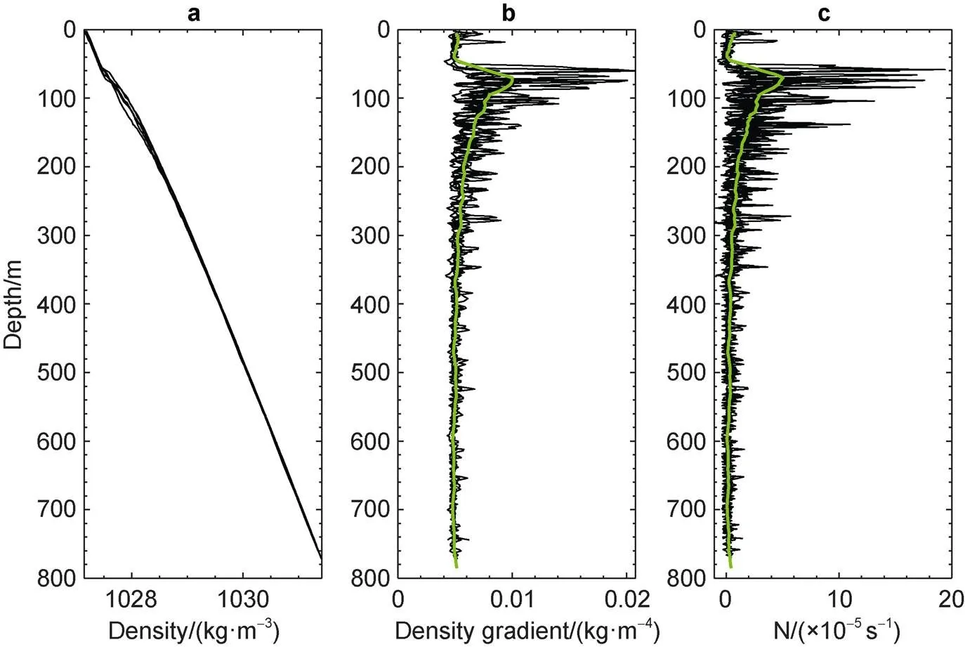
Figure 4 a, Density profiles calculated from the legacy temperature and salinity data shown in Figure 2; b, Vertical density gradient calculated from the density in (a); The black solid lines are measured data, and the green solid line is the smoothed data; c, Brunt-Väisälä frequency calculated from the density in (a). The black solid lines are measured data, and the green solid line is the smoothed data.

Figure 5 Monthly mean sea surface temperature (a) and velocity (b) in February 1993. The solid black line is seismic line AP25. The black arrow indicates the reference velocity. The temperature and velocity data is from CMEMS.

Figure 6 a, Distribution of shelf break front picked from the seismic profile; b, The slope angle of the shelf break front.

Shelf-break front is frontal formations where cross-shelf waters encounter slope waters from the deeper oceans, often associated with upwelling (Condie, 1993; Gawarkiewicz and Plueddemann, 2020). The seasonally transitional features are sites of high temperature, salinity, and density gradients and often of high productivity where deep upwelled water contributes high nutrients.

5 Discussion

5.1 The influence on climate and ecosystem

According to the traditional view, ablation from Antarctic ice shelves occurs mostly by iceberg calving, with basal melting only contributing 10%–28% of the total mass loss (Jacobs et al., 1992). New research indicated that ocean waters melting the undersides of Antarctic ice shelves are responsible for most of the continent’s ice shelf mass loss (Rignot et al., 2013). In the Southern Ocean, the lower CDW, which are warmer than upper ASW and WW, can transport warm water across the shelf and intrude the ice shelves. The cross-shelf transportation of warm water may increase the melting of the foundation, thereby promoting splitting glacier and ice loss (Rignot et al., 2008). The anticyclonic eddy can carry warm core water for a long distance, while almost maintaining the properties of core water (Mcwilliams, 1985). Thus, apart from the lower warm CDW, the core water mass that is warmer than surface water and surrounding water will melt the undersides of Antarctic ice shelves (Gunn et al., 2018). In this work, this submesoscale eddy may trap warm core water. This may promote the melting of sea ice.

Submesoscale processes including submesoscale eddies and fronts are particularly relevant to phytoplankton productivity because the time scales on which they act are similar to those of phytoplankton growth (Zhang et al., 2019). The vertical secondary circulations in the fronts and the lateral boundaries of the eddies tend to destroy the lateral buoyancy gradient and restore the oceanic density stratification, which can induce upwelling (Capet et al., 2008; McWilliams et al., 2009; McWilliams, 2016) (Figure 7). The upwelling can transport nutrients from the bottom to the surface. Especially in the shelf-break front zone, there is almost the highest primary productivity (Gawarkiewicz and Plueddemann, 2020). A study in the Cosmonaut Sea found that half of the cumulative krill density across that survey was found within 80 km of the 1000 m isobath (the shelf break), and 40% within 40 km (Jarvis et al., 2010). Many researchers found that the zooplankton and related biological quantity are quite high near the shelf break of the SSI (Corzo et al., 2005; Reiss et al., 2008; Joiris and Dochy, 2013). As shown in Figure 8a, chl-concentration observed from MODIS-Terra near shelf-break is obviously higher than that north of shelf.

Figure 7 Sketch of vertical secondary circulations of the anticyclonic eddy (left) and the shelf break front (right).

5.2 Limitations of seismic data

In this study, seismic data has some limitations. As shown in Figure 8b, there may be some thin ice covering the sea surface, which will increase the difficulty of seismic acquisition, and reduce the quality of seismic data. In addition, the minimum distance between the shot and geophone is 863 m, which is too far to acquire high signal-noise ratio data.

The difference of water columns at middle and low latitudes is mainly caused by the temperature difference, while in polar regions, it is mainly caused by salinity difference. The seismic reflection coefficients are more affected by temperature than salinity (Ruddick et al., 2009). Therefore, seismic oceanographic imaging in polar regions will be more difficult. Sea ice cover will also have a certain impact on seismic acquisition and data signal-to-noise ratio. We may use a larger capacity airgun to collect seismic data in the ice-free period as far as possible to improve the signal-to-noise ratio.

6 Conclusion

Using legacy multichannel seismic data AP25 of cruise EW9101 acquired on the northeast of SSI in February 1991, we identified the oceanic submesoscale eddy with the horizontal scale ～4 km and a steep shelf break front that has variable dip angles from 5oto 10o. The submesoscale eddy is an anticyclonic eddy, which carries warm core water, can accelerate ice shelf melting. The upwelling induced by shelf break front may play an important role in transporting nutrients to the sea surface. The seismic images with very high lateral resolution may provide a new insight to understand the submesoscale and even small-scale oceanic phenomena in the interior.

Figure 8 a, The monthly mean Chl-concentration around SSI in February 2001 from MODIS-Terra. The black line is seismic line AP25. Note that the color scale is displayed in logarithm. b, Thedaily area fraction of sea ice around SSI on February 22, 2003 from NEODAAS.

Acknowledgements We thank the cruise members of R/V Maurice Ewing cruise EW9101 for acquiring the seismic data. The seismic data is provided by MGDS (https://www.marine-geo.org/tools/search/Files. php?data_set_uid=6923). The legacy CTD data is provided by NCEI (https://www.ncei.noaa.gov/access/global-temperature-salinity-profile- programme/gwi.html). The Chl-data is provided by NASA’s Ocean Color Web (https://oceancolor.gsfc.nasa.gov/). The sea ice data is provided by NEODAAS (https://www.neodaas.ac.uk/Home). This work was financially supported by National Polar Special Program “Impact and Response of Antarctic Seas to Climate Change” (Grant nos. IRASCC 01-03-01, 01-03-02), and is funded by the National Natural Science Foundation of China (Grant no. 41976048), and the National Key R&D Program of China (Grant no. 2018YFC0310000). We would like to thank four anonymous reviewers, and Guest Editor Prof. Jiuxin Shi, for their valuable suggestions and comments thatimproved this article.

Biescas B, Sallarès V, Pelegrí J L, et al. 2008. Imaging meddy finestructure using multichannel seismic reflection data. Geophys Res Lett, 35(11): L11609, doi:10.1029/2008gl033971.

Capet X, McWilliams J C, Molemaker M J, et al. 2008. Mesoscale to submesoscale transition in the California Current system. part II: frontal processes. J Phys Oceanogr, 38(1): 44-64, doi:10.1175/ 2007jpo3672.1.

Chelton D B, deSzoeke R A, Schlax M G, et al. 1998. Geographical variability of the first baroclinic Rossby radius of deformation. J Phys Oceanogr, 28(3): 433-460, doi:10.1175/1520-0485(1998)028<0433: gvotfb>2.0.co;2.

Chelton D B, Schlax M G, Samelson R M, et al. 2007. Global observations of large oceanic eddies. Geophys Res Lett, 34(15): L15606, doi:10.1029/2007gl030812.

Condie S A. 1993. Formation and stability of shelf break fronts. J Geophys Res, 98(C7): 12405, doi:10.1029/93jc00624.

Corzo A, Rodríguez-Gálvez S, Lubian L, et al. 2005. Spatial distribution of transparent exopolymer particles in the Bransfield Strait, Antarctica. J Plankton Res, 27(7): 635-646, doi:10.1093/plankt/fbi038.

Dong C M, McWilliams J C, Liu Y, et al. 2014. Global heat and salt transports by eddy movement. Nat Commun, 5: 3294, doi:10.1038/ ncomms4294.

Dong C Z, Song H B, Bai Y, et al. 2010. The latest development of Seismic Oceanography. Prog Geophys, 25(1): 109-123 (in Chinese with English abstract).

Gawarkiewicz G, Plueddemann A J. 2020. Scientific rationale and conceptual design of a process-oriented shelfbreak observatory: the OOI Pioneer Array. J Oper Oceanogr, 13(1): 19-36, doi:10.1080/1755876X.2019.1679609.

Gorman A R, Smillie M W, Cooper J K, et al. 2018. Seismic characterization of oceanic water masses, water mass boundaries, and mesoscale eddies SE of New Zealand. J Geophys Res Oceans, 123(2): 1519-1532, doi:10.1002/2017jc013459.

Gula J, Blacic T M, Todd R E. 2019. Submesoscale coherent vortices in the Gulf Stream. Geophys Res Lett, 46(5): 2704-2714, doi:10.1029/ 2019gl081919.

Gunn K L, White N, Caulfield C C P. 2020. Time-lapse seismic imaging of oceanic fronts and transient lenses within south Atlantic Ocean. J Geophys Res Oceans, 125(7): e2020JC016293, doi:10.1029/2020jc 016293.

Gunn K L, White N J, Larter R D, et al. 2018. Calibrated seismic imaging of eddy-dominated warm-water transport across the Bellingshausen Sea, Southern Ocean. J Geophys Res Oceans, 123(4): 3072-3099, doi:10.1029/2018jc013833.

Holbrook W S, Fer I. 2005. Ocean internal wave spectra inferred from seismic reflection transects. Geophys Res Lett, 32(15): L15604, doi:10.1029/2005gl023733.

Holbrook W S, Páramo P, Pearse S, et al. 2003. Thermohaline fine structure in an oceanographic front from seismic reflection profiling. Science, 301(5634): 821-824, doi:10.1126/science.1085116.

Huang X H, Song H B, Bai Y, et al. 2013. Estimation of geostrophic velocity from seismic images of mesoscale eddy in the South China Sea. Chin J Geophys, 56(1): 181-187 (in Chinese with English abstract).

Jacobs S S, Helmer H H, Doake C S M, et al. 1992. Melting of ice shelves and the mass balance of Antarctica. J Glaciol, 38(130): 375-387, doi:10.3189/s0022143000002252.

Jarvis T, Kelly N, Kawaguchi S, et al. 2010. Acoustic characterisation of the broad-scale distribution and abundance of Antarctic krill () off East Antarctica (30-80°E) in January-March 2006. Deep Sea Res Part II Top Stud Oceanogr, 57(9-10): 916-933, doi:10.1016/j.dsr2.2008.06.013.

Joiris C R, Dochy O. 2013. A major autumn feeding ground for fin whales, southern fulmars and grey-headed albatrosses around the South Shetland Islands, Antarctica. Polar Biol, 36(11): 1649-1658, doi:10.1007/s00300-013-1383-8.

McWilliams J C. 1985. Submesoscale, coherent vortices in the ocean. Rev Geophys, 23(2): 165, doi:10.1029/rg023i002p00165.

McWilliams J C. 2016. Submesoscale currents in the ocean. Proc R Soc A, 472(2189): 20160117, doi:10.1098/rspa.2016.0117.

McWilliams J C, Colas F, Molemaker M J. 2009. Cold filamentary intensification and oceanic surface convergence lines. Geophys Res Lett, 36(18): L18602, doi:10.1029/2009gl039402.

Nakamura Y, Noguchi T, Tsuji T, et al. 2006. Simultaneous seismic reflection and physical oceanographic observations of oceanic fine structure in the Kuroshio extension front. Geophys Res Lett, 33(23): L23605, doi:10.1029/2006gl027437.

Nurser A J G, Bacon S. 2014. The Rossby radius in the Arctic Ocean. Ocean Sci, 10(6): 967-975, doi:10.5194/os-10-967-2014.

Orsi A H, Whitworth T, Nowlin W D. 1995. On the meridional extent and fronts of the Antarctic Circumpolar Current. Deep Sea Res Part I Oceanogr Res Pap, 42(5): 641-673, doi:10.1016/0967-0637(95) 00021-W.

Pingree R D, Le Cann B. 1992. Three anticyclonic slope water oceanic eDDIES (SWODDIES) in the Southern Bay of Biscay in 1990. Deep Sea Res A Oceanogr Res Pap, 39(7-8): 1147-1175, doi:10.1016/0198- 0149(92)90062-X.

Pinheiro L M, Song H B, Ruddick B, et al. 2010. Detailed 2-D imaging of the Mediterranean outflow and meddies off W Iberia from multichannel seismic data. J Mar Syst, 79(1-2): 89-100, doi:10.1016/j.jmarsys.2009.07.004.

一是加快雨洪资源利用，着力提升现代水网保障能力。加快南水北调配套工程建设，开工建设引黄济青改扩建工程。积极推进雨洪资源利用，先期规划实施一期工程18座大中型水库增容，新建8座山丘区水库、6座地下水库和32座平原水库，以及沂沭河洪水调配东线工程和东平湖增容工程，努力提高水资源供给能力。

Reiss C S, Cossio A M, Loeb V, et al. 2008. Variations in the biomass of Antarctic krill () around the South Shetland Islands, 1996–2006. ICES J Mar Sci, 65(4): 497-508, doi:10.1093/icesjms/ fsn033.

Rignot E, Bamber J L, van den Broeke M R, et al. 2008. Recent Antarctic ice mass loss from radar interferometry and regional climate modelling. Nature Geosci, 1(2): 106-110, doi:10.1038/ngeo102.

Rignot E, Jacobs S, Mouginot J, et al. 2013. Ice-shelf melting around Antarctica. Science, 341(6143): 266-270, doi:10.1126/science.1235798.

Ruddick B, Song H B, Dong C Z, et al. 2009. Water column seismic images as maps of temperature gradient. Oceanography, 22(1): 192-205, doi:10.5670/oceanog.2009.19.

Sallarès V, Biescas B, Buffett G, et al. 2009. Relative contribution of temperature and salinity to ocean acoustic reflectivity. Geophys Res Lett, 36: L00D06, doi:10.1029/2009gl040187.

Sheen K L, White N, Caulfield C P, et al. 2011. Estimating geostrophic shear from seismic images of oceanic structure. J Atmos Ocean Technol, 28(9): 1149-1154, doi:10.1175/jtech-d-10-05012.1.

Song H B, Chen J X, Pinheiro L M, et al. 2021. Progress and prospects of seismic oceanography. Deep Sea Res Part I Oceanogr Res Pap, 177: 103631, doi:10.1016/j.dsr.2021.103631.

Song H B, Pinheiro L M, Ruddick B, et al. 2011. Meddy, spiral arms, and mixing mechanisms viewed by seismic imaging in the Tagus Abyssal Plain (SW Iberia). J Mar Res, 69(4): 827-842, doi:10.1357/0022240 11799849309.

Tang Q S, Gulick S P S, Sun J, et al. 2020. Submesoscale features and turbulent mixing of an oblique anticyclonic eddy in the Gulf of Alaska investigated by marine seismic survey data. J Geophys Res Oceans, 125(1): e2019JC015393, doi:10.1029/2019jc015393.

Tang Q S, Gulick S P S, Sun L T. 2014. Seismic observations from a Yakutat eddy in the northern Gulf of Alaska. J Geophys Res Oceans, 119(6): 3535-3547, doi:10.1002/2014jc009938.

Yang S, Song H B, Fan W H, et al. 2021. Submesoscale features of a cyclonic eddy in the Gulf of Papagayo, Central America. Chin J Geophys, 64(4): 1328-1340, doi:10.6038/cjg2021O0204 (in Chinese with English abstract).

Zhang J C, Luo Y M, Xing J H. 2021. Seismic images of shallow waters over the Shatsky Rise in the Northwest Pacific Ocean. J Ocean Univ China, 20(5): 1079-1088, doi:10.1007/s11802-021-4581-y.

Zhang Z G, Qiu B, Klein P, et al. 2019. The influence of geostrophic strain on oceanic ageostrophic motion and surface chlorophyll. Nat Commun, 10: 2838, doi:10.1038/s41467-019-10883-w.

Zhang Z G, Wang W, Qiu B. 2014. Oceanic mass transport by mesoscale eddies. Science, 345(6194): 322-324, doi:10.1126/science.1252418.

Zhou M, Niiler P P, Zhu Y W, et al. 2006. The western boundary current in the Bransfield Strait, Antarctica. Deep Sea Res Part I Oceanogr Res Pap, 53(7): 1244-1252, doi:10.1016/j.dsr.2006.04.003.

Zhou M, Zhu Y W, Dorland R D, et al. 2010. Dynamics of the current system in the southern Drake Passage. Deep Sea Res Part I Oceanogr Res Pap, 57(9): 1039-1048, doi:10.1016/j.dsr.2010.05.012.

Zhou M X, Zhu G P. 2020. Water mass structure in the euphotic zone around south Shetland Islands, Antarctic during summer 2013. Chin J Polar Res, 32(1): 90-101 (in Chinese with English abstract).

31 March 2021;

17 February 2022;

30 March 2022

10.13679/j.advps.2021.0004

, ORCID: 0000-0001-8031-9983, E-mail: hbsong@tongji.edu.cn

: Yang S, Song H B, Zhang K.Research on submesoscale eddy and front near the South Shetland Islands (Antarctic Peninsula) using seismic oceanography data. Adv Polar Sci, 2022, 33(1): 110-118,doi:10.13679/j.advps.2021.0004