Real-Time Iterative Compensation Framework for Precision Mechatronic Motion Control Systems

Chuxiong Hu,,, Ran Zhou, Ze Wang,,, Yu Zhu,,, and Masayoshi Tomizuka,,

Abstract—With regard to precision/ultra-precision motion systems, it is important to achieve excellent tracking performance for various trajectory tracking tasks even under uncertain external disturbances. In this paper, to overcome the limitation of robustness to trajectory variations and external disturbances in offline feedforward compensation strategies such as iterative learning control (ILC), a novel real-time iterative compensation(RIC) control framework is proposed for precision motion systems without changing the inner closed-loop controller.Specifically, the RIC method can be divided into two parts, i.e.,accurate model prediction and real-time iterative compensation.An accurate prediction model considering lumped disturbances is firstly established to predict tracking errors at future sampling times. In light of predicted errors, a feedforward compensation term is developed to modify the following reference trajectory by real-time iterative calculation. Both the prediction and compensation processes are finished in a real-time motion control sampling period. The stability and convergence of the entire control system after real-time iterative compensation is analyzed for different conditions. Various simulation results consistently demonstrate that the proposed RIC framework possesses satisfactory dynamic regulation capability, which contributes to high tracking accuracy comparable to ILC or even better and strong robustness.

I. INTRODUCTION

MOTION control has been extensively applied in the modern precision/ultra-precision industry [1]–[5]. For many precision mechatronic equipments, such as wafer stages,CNC machine tools, linear motors, hard disk drivers, and piezoelectric actuators, accurate trajectory tracking performance is one of the most important components. In addition,due to the ubiquitous and inevitable uncertain external disturbances (e.g., dynamic cutting forces, cable disturbances)which may result in prominent deterioration of tracking accuracy, the disturbance rejection ability of the precision controller is another pivotal issue in practical applications [6],[7]. Consequently, the design of a precision motion controller with high tracking accuracy and strong disturbance rejection ability remains a significant research topic.

Recently, multiple advanced control methods have been proposed to improve the tracking performance of precision motion systems. All these methods can be divided into two categories, one of which is to design novel feedback controller structures such as adaptive robust control (ARC) [8], sliding mode control (SMC) [9], fuzzy control (FC) [10], active disturbance rejection control (ADRC) [11], etc. However, in some industrial scenarios, the practical system is equipped with a fixed feedback controller which is hard to customize.To avoid this constraint, another idea is to add extra feedforward compensation modules into the existing feedback control system [12]–[16]. Without changing the original feedback controller structure, these feedforward compensation methods can sufficiently exploit system characteristics to remedy the inherent dynamical lag and enhance closed-loop control performance, which have great potential for industrial applications.

Among various feedforward compensation ideas, iterative learning control (ILC) is one of the most effective strategies for online synthesis of the feedforward signal to achieve excellent tracking control performance. The remarkable tracking accuracy of ILC has been successfully and widely verified on different kinds of mechatronic equipments, such as wafer scanner systems [17], linear motion stages [18], tower crane systems [19], and piezoelectric actuators [20]. The main idea of ILC is to extract system characteristics from previous iteration trials to modify the control input in the next iteration trial, and ultimately obtain optimal feedforward compensation.To expand the robustness of traditional ILC for extensive applications, learning adaptive robust control (LARC) [21] and neural network learning adaptive robust control (NNLARC)[22] have been successively proposed to enhance the disturbance rejection ability. Some robust optimization methods can also be embedded in ILC for complex plant systems [23].However, standard ILC and its derivations are so sensitive to reference trajectory variations that repetitive re-iteration trials are compulsory for each new trajectory even with slight variations [24]. For practical application scenarios, it is very time-consuming to conduct the repetitive learning process.

In order to achieve both excellent tracking accuracy and great generalization for various trajectories, projection-based ILC (P-ILC) utilizes basis functions to fit the reference trajectories and known repeated disturbances, which significantly enhances generalization and robustness [17], [25]. Additionally, artificial neural networks have been employed in control engineering on account of its powerful modeling capability in recent years [26]–[30]. In [28] and [29], a gated recurrent unit (GRU) network was trained to accurately predict tracking error before implementation, and the predicted error was directly added to the reference trajectory as a feedforward structure, which achieved high tracking accuracy as ILC. A similar GRU-based method has also been proposed to fit the optimal trajectory modification of ILC [30]. Yet, in all the aforementioned GRU-based and ILC-based compensation strategies, time-consuming offline pre-implementations for network training and iteration trials are inevitable. Besides,these methods cannot suppress accidental uncertain disturbances since all the compensation terms have been definitely determined before practical implementation.

Different from those offline compensation schemes, there are also some control strategies which improve the tracking performance during real-time motion. For instance, repetitive control (RC) is an effective online learning-type method tailored for periodic trajectories, which can reduce tracking error as the operation period increases [31]–[33]. However,RC is impotent when dealing with complicated aperiodic tasks. Model predictive control (MPC) is another well-known method originating from the process industry with the advantages of strong robustness and simple implementation [34].Based on the system prediction model, the control input at each sampling time is determined by online optimization of a cost function related to input constraints or control performance (e.g., tracking error). Recently, MPC has also been applied to various precision motion systems [35], [36].Nevertheless, final tracking accuracy is indirectly limited by the weight matrix of the tracking error term in the cost function. In other words, the extent to which the error can be reduced cannot be explicitly obtained when designing the MPC controller.

In this paper, in order to improve dynamic regulation capabilities and overcome the limitation of robustness to trajectory variations and external disturbances in offline feedforward compensation strategies, a novel real-time iterative compensation (RIC) framework is proposed for precision motion systems without changing the inner closed-loop controller.Specifically, an accurate prediction model is established for linear closed-loop motion systems to predict tracking errors at future sampling times. An extra perturbation term is added in the prediction model to further suppress the influence of lumped external disturbances. Based on the predicted errors,an iterative compensation scheme is utilized to modify the future reference trajectories. The stability and convergence of the entire control system is theoretically analyzed and proved.Comparative simulation investigations have validated the effectiveness of the proposed RIC framework, and its advantages can be summarized as follows:

1) The established prediction model provides a precise approximation of the actual motion system, which can accurately predict future tracking errors even under external disturbances. Subsequently, the predicted error is iteratively developed as a trajectory compensation for tracking accuracy improvement.

2) The proposed RIC framework is an online method that both prediction and compensation processes are merely finished in a real-time sampling period. This mechanism endows the RIC method with dynamic regulation capability.Consequently, it not only achieves high tracking accuracy comparable to ILC or even better, but also possesses strong robustness to trajectory variations and external disturbances.

3) RIC is a feedforward compensation scheme that does not change the inner feedback controller structure. Additionally,abundant but indispensable pre-implementations in GRU/ILCbased offline compensation strategies are omitted. Therefore,it is simple and efficient to be conducted in practical scenarios.

II. PROBLEM FORMULATION AND SYSTEM PREDICTION

A. System Description

In this paper, single input single output (SISO) systems representing one-axial motion systems are considered. A standard closed-loop feedback control architecture for precision motion systems is shown in Fig. 1.Gcis the feedback controller,Gpis the plant model,ris the reference trajectory,pis the actual output position,eis the tracking error,uis the control input determined by feedback controller,dis the perturbation onu, andnmis the position measurement noise.

Fig. 1. Block diagram of standard closed-loop feedback control.

Without loss of generality, the relationship between the control inputuand the actual output positionpof the plant model can be expressed as

where the polynomialsD(z),N(z) can be expressed as

andw≥vandw,v∈N+.kdenotes the sampling time.Essentially,Gp(z)=N(z)/D(z) is the plant transfer function.

The feedback controller can also be described in the form of the transfer function. For instance, the widespread PID feedback controller is expressed as

whereTsis the sampling period.kp,ki,kdare the proportional gain, integral gain, and derivative gain, respectively.

According to (1) and (3), the reference-position relationship of the closed-loop system in Fig. 1 is

D′(z)N′(z)

where the polynomials and are andq=max(w+1,v+2),l=v+2.Nc(z) andDc(z) are the numerator and denominator of PID controller (3).αi,βj(i=1,...,q;j=1,...,l)can be derived by the parameters of the feedback controller and plant model.δis the lumped perturbation term caused by external disturbanced.

For precision motion systems, the main target is to minimize the tracking errore=r−psuch that the output position can precisely track various reference trajectories even in the existence of uncertain disturbancesd. The proposed RIC framework is elaborated as follows.

B. Accurate Prediction Model

In order to accurately predict tracking errors at future sampling times, the reference-position relationship is utilized to establish the prediction model. The difference equation derived from (4) is

Letx(k) be the state vector at timekTs. Supposeq=l, then(6) can be converted to state space equations (SSE) expressed as

In SSE (7), ϵ(k) is the perturbation vector,A,B,Care the state matrix, input matrix, and output matrix respectively, i.e.,

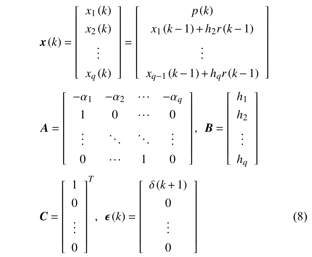
andhican be recursively calculated by

Definition 1(Prediction horizonNp):The prediction horizon is the number of future time intervals to be predicted.That is, at current sampling timekTs, state vectors from(k+1)Tsto (k+Np)Tswill be predicted.

A system prediction model is established in the light of SSE(7). Supposedenotes the predicted variable, state vectors in the prediction horizon can be recursively derived by

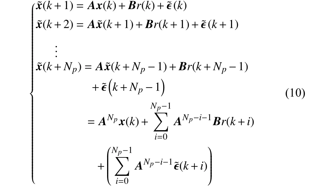
where the current state vectorx(k) and future reference trajectoriesr(k+i)(i=0,1,...,Np−1) are known. However,all the perturbations at future sampling times are unattainable in advance. To make (10) feasible for prediction, some common assumptions about unknown perturbations are given [37],[38].

Assumption 1:The perturbation is almost equal in adjacent periods and the actual perturbation at the last moment is used to approximate the perturbation at the current moment, i.e.,

Assumption 2:The predicted perturbation at each moment in the prediction horizonNpis constant, i.e.,

Assumption 3:The perturbation at each sampling time is bounded and satisfies the Lipschitz condition, i.e.,

wheret1,t2denote two time instants,Lis a Lipschitz constant.

Based on Assumptions 1 and 2, the unknown perturbation vectors in prediction horizon are assumed as

Substituting (10), (14) into the output equation in SSE (7),the prediction model of output position is

Additionally, the prediction deviationε(the difference between actual value and predicted value) can be deduced by

Based onAssumption 3, it can be obtained that

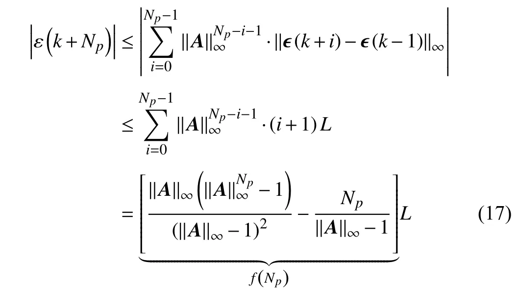
where //A//∞is the ∞-norm ofA. Obviously,f(Np) is an increasing function with respect toNpsince //A//∞>1, and the prediction deviation is bounded in the sense of|ε(k+Np)|≤f(Np)L. This inequality also reveals that the prediction accuracy will significantly decrease asNpincreases due to the inevitable perturbation accumulation. For practical application,Npis normally selected as a small value and the Lipschitz constantLis also a sufficiently small value that satisfiesL=O()[37]. Consequently, the accurate system prediction can be achieved under these conditions.

C. Unbiased Parameter Estimation

To guarantee the prediction accuracy, the prediction model can be obtained by closed-loop system identification. The closed-loop system (4) is in the form of ARMAX time series model, whose parameters can be identified by the following recursive extended least squares (RELS) algorithm [39].

Suppose ϑ ∈Rq+l+v+1is the system parameter vector and φ(k)∈Rq+l+v+1is the information vector, i.e.,

where ϕi(i=1,...,v+1) are polynomial coefficients ofDc(z)N(z)in (4). Consequently, (4) is rewritten as

In (19), the information vector φ(k) contains unmeasurable disturbancesd(k−1),...,d(k−v−1). A feasible alternative is to approximate these true disturbances with their estimation terms, i.e.,

According to [39], if the disturbanced(k) is a white noise sequence with zero mean and the persistent excitation condition holds, is an unbiased estimation of nominalϑ, i.e.,

III. REAL-TIME ITERATIVE COMPENSATION

A. Real-Time Iterative Compensation Scheme

Tracking errore(k) is the difference between the actual position and the reference trajectory. Without any compensation scheme applied, the initial predicted tracking error of the closed-loop system at (k+Np)Tsis

According to (15), the predicted position at (k+Np)Tsis directly related to future reference trajectoriesr(k+i)(i=1,2,...,Np−1). Therefore, a reasonable design of reference trajectory compensation term can make the actual output position closer to the desired one. Based on this principle, a real-time iterative compensation strategy is proposed to reduce the tracking error.

Definition 2(Compensation horizonNc):Based on prediction results, the compensation horizonNc≤Np−1 is the future sampling time when the compensation term will be added to the reference trajectory.

If a compensation termcis added to the reference trajectory at (k+Nc)Ts, the output position at (k+Np)Tswill change accordingly due to the reference trajectory modification.Accordingtothepredictionmodel (10),(15),thequantitative relationshipbetweentheposition increment∆pand the compensation termc(k+Nc) can be expressed as

whereξis a constant coefficient related to system matricesA,B,Cand algorithm parametersNp,Nc.

After compensation, the tracking error is updated by

In order to reduce tracking error and improve the tracking accuracy, a real-time iterative compensation scheme is proposed for precision motion systems. The framework of this scheme is shown in Fig. 2. In general, the recursion formula of the compensation term in adjacent iteration steps is designed as

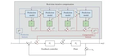
Fig. 2. Structure of the proposed RIC method.

where the superscripti∈N is the iteration step andγis the constant compensation gain. For the initial condition,c(0)=0,eˆ(0)=. Consequently, the compensation term in the first iteration is designed as

The tracking error after the first iteration will be

In the second iteration,eˆ(1)is also added to the first compensation termc(1)and the final compensation term becomes

Accordingly, the tracking error after the second iteration will be

Following the above iterative approach, the final compensation termc(n)at thenth iteration can be expressed as:

Consequently, the ultimate tracking error becomes

The compensation gainγis artificially determined to guarantee the effectiveness of the proposed method. According to (31) and (32), if the compensation gain is set to γ1=1,the final compensation term at thenth iteration can be expressed as

and the tracking error after compensation becomes

Obviously, this compensation strategy can significantly reduce the tracking error when ξ →1, while it has almost no effect when ξ →0. To make up for this defect, an alternative compensation gain is selected as γ2=(1−ξ)/ξ. Accordingly,the compensation term becomes

and the tracking error after compensation is

Opposite of the condition where γ=γ1=1, ifγ=γ2=(1−ξ)/ξ, the tracking error will significantly decrease when ξ →0 but have almost no effect when ξ →1. Ultimately, the compensation gain is determined byξ, i.e.,

Accordingly, the final compensation term is deduced to

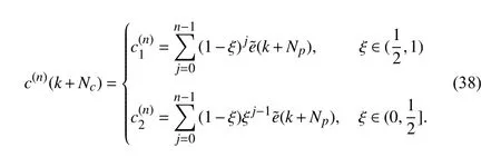
The general idea of the RIC method is summarized as follows. At current timekTs, future tracking errors in the prediction horizon (from (k+1)Tsto (k+Np)Ts) can be accurately predicted. Subsequently, the compensation term at(k+Nc)Ts(Nc≤Np−1)is iteratively calculated based on the predicted tracking error at (k+Np)Ts. This process is repeated in each real-time sampling period. Therefore, the actual closed-loop system input at each sampling time is the sum of initial reference trajectory and the corresponding compensation term.

Remark 1:The system prediction model (15) is a precise approximation of the actual motion system and the prediction deviation inevitably exists. According to (17), asNpincreases,the prediction accuracy will diminish monotonously due to the continuous accumulation of previous prediction deviations. In this paper, to ensure prediction performance and simplify the RIC method, the prediction horizon is set asNp=2 while the compensation horizon isNc=Np−1=1.

Remark 2:In theory, the tracking error can be completely eliminated ifeˆ=0 according to (25), and the corresponding compensation termc∗=ξ−1eˆ is defined as theoretically optimal. However, it is unreachable in practice. If the compensation term is directly determined byeˆ=0, useless interference signals and high-frequency noises will also be fully compensated, which results in performance deterioration,high-frequency oscillation and even system instability. Therefore, the above iterative compensation scheme is implemented to asymptotically reduce tracking error.

B. Stability and Convergence Analysis

Different from offline compensation strategies, the compensation term is a function of the real-time output position.Therefore, the stability of the entire system should be reanalyzed even though the inner controller structure is unchanged. Meanwhile, the tracking error should keep decreasing as the iteration stepnincreases, and the compensation term at any sampling time should converge to one that is optimal with minimal tracking error. The following theory gives the sufficient condition for the stability and convergence.

Lemma 1:Let a matrixM∈RN×Nand ∀σ>0 be given.There is an induced matrix norm // •//isuch that//M//i≤ρ(M)+σ. Here, ρ(M) is the spectral radius ofM.

Proof:SeeLemma 5.6.10in [40]. ■

Theorem 1:If the system parameter β1satisfies

the stability of the entire control system is guaranteed. Besides, the tracking error will keep decreasing and the compensation termatanysamplingtimekTswillmonotonously convergetotheoptimaltermc∗(k) astheiteration stepn→∞.

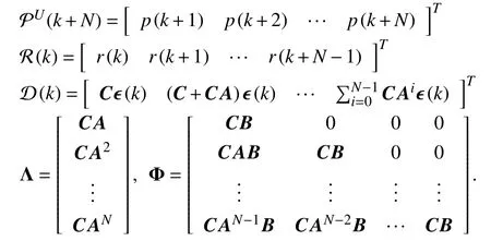
Proof:For a reference trajectory withNpoints, at any sampling timekTs, the following position sequence without compensation can be expressed as:

where PU(k+N)∈RN×1denotes the uncompensated position sequence,x(k)∈Rq×1is the current state vector defined in (8),R(k)∈RN×1is the reference trajectory sequence,D(k)∈RN×1

Λ ∈RN×qΦ ∈RN×Nis the lumped perturbation sequence, , are constant coefficient matrices whose elements are related to control system parameters, i.e.,

In contrast, the position sequence after compensation with RIC method can be expressed as

where C(n)(k) is the compensation sequence composed of compensation terms for each trajectory point, i.e.,

According to (38), the compensation term at each sampling time is proportional to the predicted tracking error, i.e.,

where κnis the proportional coefficient related to the iteration stepnand can be derived from (38) as

The recursion formula of the compensation termccan be deduced by substituting (25) into (42), i.e.,

which is equivalent to

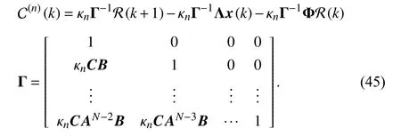
Obviously, Γ ∈RN×Nis a lower triangular matrix that is non-singular. Substituting (40), (45) into (41), the compensated position sequence can be expressed as

Suppose E=R−P is the tracking error sequence, the relationship between the compensated error sequence ECand uncompensated error sequence EUis

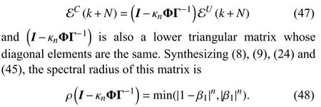
It is obvious that ρ<1 if the system parameter β1satisfies thesufficientcondition0<β1<1.Therefore, letσ=(1−ρ)/2>0begiven,ECandEUsatisfythefollowing trigonometric inequality according toLemma 1, i.e.,

For the closed-loop system without the RIC method applied,stability is guaranteed by the feedback controller, so the uncompensated tracking error sequence EUis definitely bounded. According to (49), the induced norm of the compensated tracking error sequence is also bounded. In other words,the tracking error cannot be infinite and the stability of the entire system after compensation is still guaranteed.

In terms of convergence analysis, the optimal compensation term in theory is determined by assuming (25) equal to 0, i.e.,

According to (43), the compensation terms under different iteration stepnsatisfies

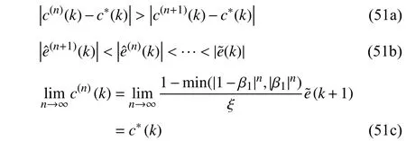
which means that the tracking error will monotonously decrease asnincreases, and the compensation term converges to the optimal term asn→∞. ■

It should be pointed out that the sufficient condition (39) is merely related to the system parameter β1which has been determined after the design of initial closed-loop control system. In other words, (39) inTheorem 1is a “passive”condition where there is no tuning knob for the designer. In order to “actively” guarantee the stability and convergence of the proposed RIC method no matter if condition (39) is satisfied, an iteration-varying compensation gain is designed and the results are clarified as the following theorem.

Theorem 2(Active condition):If β1does not satisfy the sufficient condition (39), the compensation gain γ can be designed as an iteration-varying function γiin the form of

whereidenotes the iteration step and η>0 is an attenuation factor that satisfies

With this configuration, the stability and convergence described inTheorem 1can be still guaranteed.

Proof:By replacing the constant compensation gainγwith the iteration-varying compensation gain γi, the recursion formula (26) under the conditionNp=2,Nc=1 can be rewritten as

and the initial condition becomesc(1)(k)=γ1e˜(k+1).

Similar to (47), the tracking error sequences in adjacent iteration stepsiandi−1 satisfy

where the coefficient matrixI−γiΦΓ−1(γi) is

Consequently, the relationship between the compensated tracking error sequence afternth iteration and the uncompensated one can be derived as

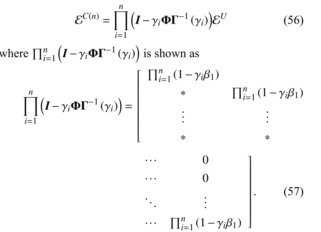
Obviously, the spectral radius of this matrix is

Substituting the iteration-varying compensation gain (52)into (58),ρcan be updated as

Based onLemma 1, suppose the spectral radius satisfies ρ((I−γiΦΓ−1(γi)))<1, the following inequality should be guaranteed for an arbitrary iteration stepn∈N, i.e.,

The above inequality provides the demanding range of attenuation factorη. Synthesizing (52), (54) and (25), the final compensation termc(n)(k) at thenth iteration and the compensated tracking erroreˆ(n)(k) can be derived as

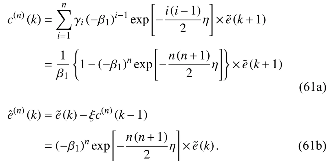
According to (61a), the proportional coefficient κndefined in (42) becomes

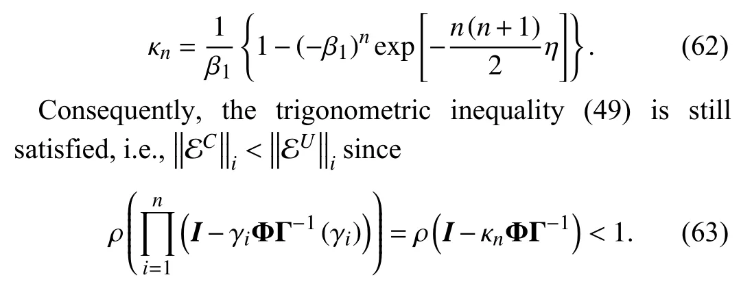
The same relationship as shown in (51) can also be obtained under this condition, i.e.,

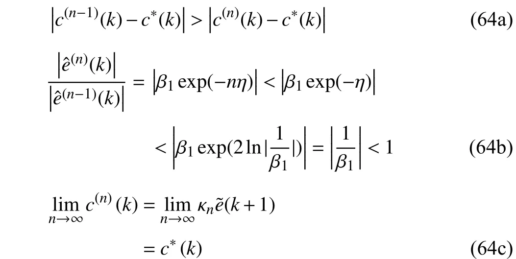
which means that the tracking error will monotonously decreaseasnincreases, andthe compensation term converges to theoptimaloneasn→∞.■In essence,Theorem 2is a complement toTheorem 1since β1is completely determined by the feedback controller and plant model. Therefore, the proposed RIC method is impotent if the closed-loop feedback system does not satisfy the sufficient condition inTheorem 1. The iteration-varying compensation gain inTheorem 2extends the applicability of the RIC method to any closed-loop system. Additionally, it should be pointed out that the iteration-varying compensation gain (52) designed inTheorem 2is not a unique choice to actively guarantee the stability and convergence of the entire control system. Instead, appropriate functions that simultaneously satisfy (63) and (64) are available in this method. The exponential function utilized in this paper is a satisfying alternative.

C. Bounded Error Characteristic With Randomized Noises

For the stability and convergence analysis in the previous section, the prediction model is assumed to be definitely accurate so that the compensated tracking error will asymptotically converge to zero. However, according to (17), the prediction deviation inevitably exists in the presence of system uncertainty and randomized disturbance. Taking these factors into account, the following analysis reveals that the tracking error compensated by the RIC method is still bounded.

WithNp=2 andNc=1, the recursive formula (26) of the compensation term can be rewritten as

Suppose that ω(i)and ν(i)denote the randomized state noise and the randomized output noise, respectively. Therefore, the closed-loop system dynamics with RIC method applied can be expressed as

In (66),A,B,ω(i)(k),ν(i)(k) satisfy the properties and bounds stated as the following assumption.

Assumption 4:For simplicity, let //•// be the 2-norm of matrices or vectors.

2) For the ideal condition without ω(k),ν(k) in (66), the zero-error-tracking can be achieved by a bounded state sequence {x∗(k)}, a bounded compensation sequence{c∗(k)}andabounded outputsequence{p∗(k)}.

Definition 3(α-norm):The α-norm (α >1) is defined for a positive real function τ :N →R as

In the sense ofα-norm, the following theorem guarantees the bounded system output with the RIC method applied even in the presence of randomized noises.

Lemma 2:Given a difference inequality

wherey(•) and χ(•) are scalar functions ofk≥0, and g is a positive constant. Then, fork≥1,

Proof:SeeLemmain [41]. ■

Theorem 3:If the sufficient condition (39) ofTheorem 1and theAssumption 4hold, the compensated tracking error by

RIC is still bounded in the presence of system noises ω ,ν, i.e.,

Proof:Subtractingc∗(k) from both sides of (65) yields

where ∆λ(i)=λ∗−λ(i)for λ ∈{x,c,p}. For the ideal condition where there are no randomized noises ω,ν in (66),x∗andc∗satisfy

Substituting (72) into (71), one can obtain that

Taking the 2-norms of both sides of (73) and applying the triangular inequality, the following inequality is obtained as:

where ρ ∈(0,1) is defined in (48) and ∆x(i)(k) satisfies

The triangular inequality can also be extended to (75), i.e.,

According toLemma 2, it can be obtained from (76) that

and the relationship between ||∆c(i+1)(k)||,||∆c(i)(k)|| can be deduced by substituting (77) to (74), i.e.,

Multiplying both sides of (78) by ( 1/α)kwhere the constantαsatisfies α >max{1,}, (78) can be extended in the sense ofα-norm based on Definition 3, i.e.,

Then, (79) is a contraction in the sense of | |∆c(i)||α. With the iteration stepi→∞, | |∆c(i)||αis still bounded by

Algorithm 1 Real-Time Iterative Compensation (RIC)

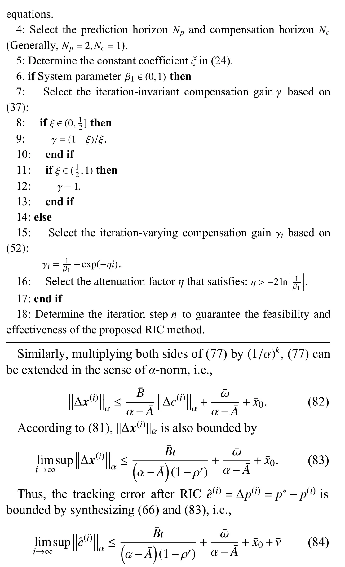
which is equivalent to (70). ■

Essentially,Theorem 3complements the stability and convergence analysis in the previous part. For the ideal condition that randomized noises ω ,ν are assumed to be 0,Theorem 3is definitely equivalent toTheorem 1andTheorem 2. More importantly,Theorem 3guarantees the bounded system output even with the existence of randomized noises.

D. General Framework of RIC Method

In this part, the general framework of the proposed RIC method has been concluded as shown in Algorithm 1. Firstly,qandlin (4) is determined according to the linear transfer function of the plant model derived by dynamics analysis.Then, system parameters αi,βj(i=1,...,q;j=1,...,l) can be obtained by closed-loop system identification. Based on the identification results, the prediction model (10), (15) can be obtained as a precise approximation of the practical system.Afterwards, the prediction horizonNpand the compensation horizonNcare selected to ensure the prediction accuracy and simplify the algorithm. Hence, the compensation gainγis determined according toTheorem 1orTheorem 2. Finally, the iteration stepnof the iterative calculation process is artificially selected to guarantee the feasibility and effectiveness of the proposed RIC method.

Remark 3:It should be pointed out that the generation process of trajectory compensation term in the RIC method is definitely different from ILC. Given a certain trajectory tracking task implementation, for ILC, offline iteration trials need to be conducted on practical devices in advance where the compensation term is derived from the practical data. In contrast, the compensation term in RIC method is online generated by the established prediction model during the operation of motion systems rather than determined in advance by iterative experiments. Thus, the proposed RIC method is more flexible and efficient since it possesses dynamic regulation capability and omits abundant compulsory iteration trials in ILC.

Remark 4:Theoretically, the tracking error will continuously decrease as the iteration stepnincreases. However, it is not feasible to setnto an arbitrary large value in practice since several factors will limit the upper bound ofn:

1)Calculation Burden:All the iterative calculations must be finished during one sampling period. That is, the selection of iteration stepnmust satisfy real-time feasibility.

2)Measurement Resolution and Noise:The measurement resolution and noise in practical systems will limit the reachable tracking performance. After sufficient iterative compensation, the tracking error will not continue to decrease even ifnkeeps increasing.

IV. SIMULATION INVESTIGATION

In this section, simulation investigations are carried out to validate the effectiveness of the proposed RIC method. A simulation platform of one-axial motion control system is built in Matlab/Simulink with sampling frequencyfs=5 kHz.In order to make the simulation model more similar to the practical system, the measurement resolution is considered and set as 2 nm. Some randomized measurement noises are also added. Additionally, some disturbances composed of repeated parts and non-repeated parts are injected to the control input. Two indexes are utilized to evaluate the tracking performance, i.e.,

1)erms:The root-mean-square value of the tracking error.

2)emax:The maximal absolute value of the tracking error.

Two sets of simulations are conducted to investigate tracking performance. Set 1 focuses on tracking accuracy for various reference trajectories and the disturbance rejection ability under complicated disturbances. Set 2 focuses on the feasibility of the iteration-varying compensation gain when the system parameter β1does not satisfy the condition (39).

A. Simulation Results of Set 1

In Set 1, the plant model is a second-order system, i.e.,

and the proportional, integral, derivative parameters of the PID controller are tuned askp=21060,ki=334980,kd=300.

Combining (3) and (85), the closed-loop transfer function can be derived and the order of this system is determined asq=l=4. According to the closed-loop system identification results, system parameters αi,βi(i=1,2,3,4) in (6) are

Consequently, the sufficient condition inTheorem 1is satisfied so that the compensation gainγcan be determined by(37).

In Set 1, two cases of simulation investigations are carried out. Case 1 focuses on the tracking accuracy for various reference trajectories without external disturbances while Case 2 focuses on the disturbance rejection ability under different forms of uncertain external disturbances.

Case 1 (Tracking tasks without uncertain disturbances):To provide a sufficient comparison between the proposed RIC strategy and other advanced controllers, the following four control strategies are simultaneously implemented:

C1 (GRU-NNC):A well-trained GRU network predicts the tracking error before implementation and the predicted error is compensated to the reference trajectory [28].

• Trajectory 1: Randomized NURBS

Firstly, a randomized NURBS is employed to represent general smooth trajectories as shown in Fig. 3(a). The tracking performance under C1-C4 are plotted in Fig. 3 and listed in Table I. Due to the inherent characteristics of neural networks,there must be a toplimit on the prediction accuracy of the GRU network, which ultimately limits the tracking accuracy of C1. P-ILC employs basis functions to generate the compensation term, which improves tracking accuracy to some extent.However, the selected basis functions are limited and insufficient to completely reflect the system characteristics. In contrast, S-ILC can sufficiently extract system characteristics through several iteration trials and determine the compensation term for a certain tracking task. Consequently, compared to P-ILC, S-ILC achieves better tracking performance for this reference trajectory. The proposed RIC method can accurately predict the tracking error and iteratively calculate the compensation term during real-time motion, which achieves high tracking accuracy comparable to S-ILC or even better(theermsandemaxof C4 are 89.82% and 78.68% of C2,respectively).

• Trajectory 2: Multi-sinusoidal trajectory

In order to further validate the effectiveness of the proposed method for various trajectories, a multi-sinusoidal trajectory with different frequency components is employed, i.e.,

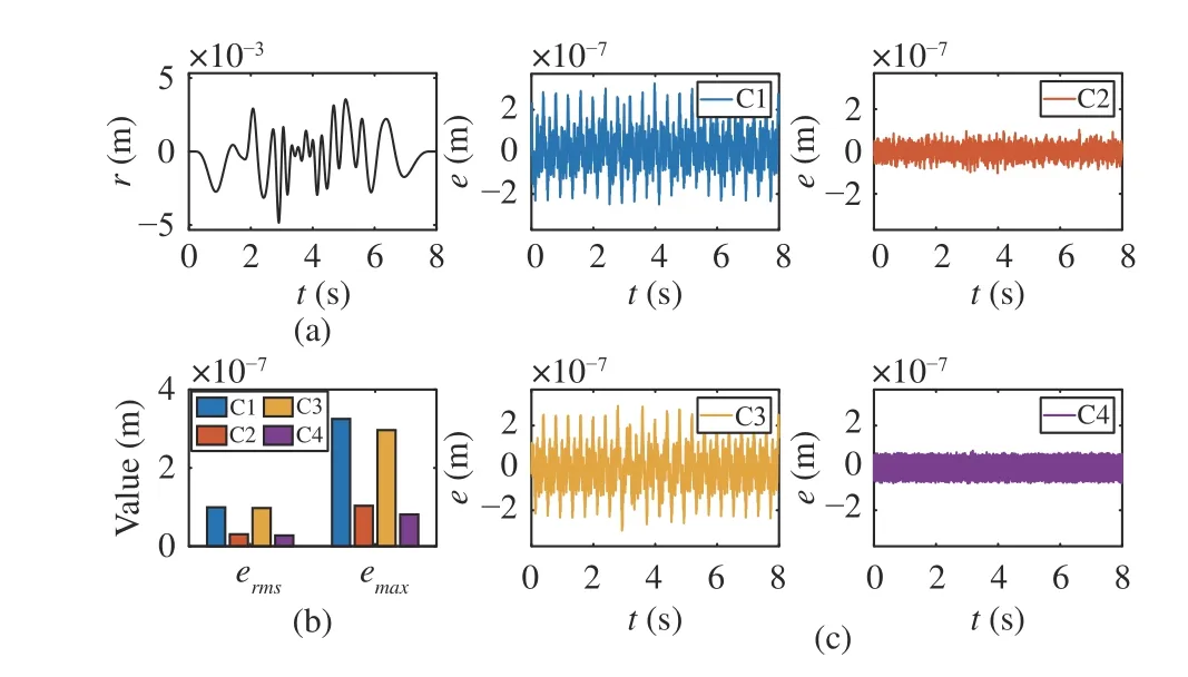
Fig. 3. Simulation results of Trajectory 1 in Case 1, Set 1. (a) Reference trajectory; (b) Performance indexes under different control strategies; (c)Tracking errors under different control strategies.

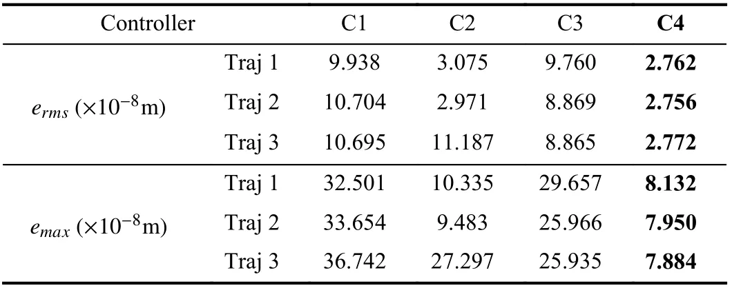
TABLE I TRACKING PERFORMANCE INDEXES OF CASE 1, SET 1

whereA1=3 mm,ω1=2πrad/s,A2=−4 mm,ω2=4 πrad/s,A3=2 mm,ω3=5 πrad/s. The reference trajectory is shown in Fig. 4(a). Tracking errors under different control strategies are plotted in Fig. 4 and listed in Table I. Obviously, the same conclusions withTrajectory 1are reached. Tracking errors of C2 and C4 are prominently less than those of C1 and C3.Additionally,ermsandemaxof C4 are 92.76% and 83.83% of C2, respectively. These results illustrate that the proposed RIC method can achieve the highest tracking accuracy for different trajectories among C1−C4.

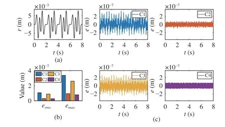
Fig. 4. Simulation results of Trajectory 2 in Case 1, Set 1. (a) Reference trajectory; (b) Performance indexes under different control strategies; (c)Tracking errors under different control strategies.

• Trajectory 3: Trajectory 2 with slight change

In order to compare the generalization for different reference trajectories of C1−C4,Trajectory 3is obtained by

slightly changing the amplitude ofTrajectory 2, i.e.,

Note that the compensation term of S-ILC is the same as that inTrajectory 2without offline re-learning. The tracking performance under C1-C4 are plotted in Fig. 5 and listed in Table I. It is obvious that GRU-NNC and P-ILC are robust to trajectory changes and their tracking performance is almost the same as those inTrajectory 2. However, S-ILC is extremely sensitive to the trajectory change, and tracking performance significantly deteriorates in spite of a slight change of reference trajectory. In contrast, the proposed RIC method still achieves high tracking accuracy, which validates its robustness to trajectory changes and generalization ability for different trajectories. All the simulation results of Case 1 consistently prove that the RIC method can achieve high tracking accuracy for tracking tasks with various reference trajectories.

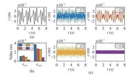
Fig. 5. Simulation results of Trajectory 3 in Case 1, Set 1. (a) Reference trajectory; (b) Performance indexes under different control strategies; (c)Tracking errors under different control strategies.

Case 2 (Tracking tasks under uncertain disturbances):In industrial scenarios, precision motion systems usually operate in the presence of various external disturbances, such as cutting forces in CNC manufacturing. To further verify the disturbance rejection ability of the proposed method, several tracking tasks under uncertain external disturbances have been conducted in this case. For comparison, the following four control strategies are simultaneously implemented:

C1:The same GRU-NNC strategy as C1 in Case 1.

C2:The same S-ILC strategy as C2 in Case 1. Note that all the external disturbances are accidentally added in the implementation. In other words, these disturbances are unavailable to be extracted by iteration trials.

C3:Compared to C2, all the external disturbances are assumed to be known before implementation. That is, these disturbances can be extracted by iteration trials. This provides an ideal benchmark but it is impossible in practice.

C4 (RIC):The proposed RIC method in this paper. The iteration step is chosen asn=3.

In this case, the randomized NURBS in Case 1 is utilized as the reference trajectory. Compared to Case 1, two different forms of external disturbances is added from 2 s to 6 s as follows.

• Disturbance 1: Sawtooth wave signal

A periodic sawtooth wave signal with the period 0.25s and amplitude ±0.004V is added as an accidental voltage perturbation shown in Fig. 6(a). Tracking performances of C1−C4 are plotted in Fig. 6 and listed in Table II.

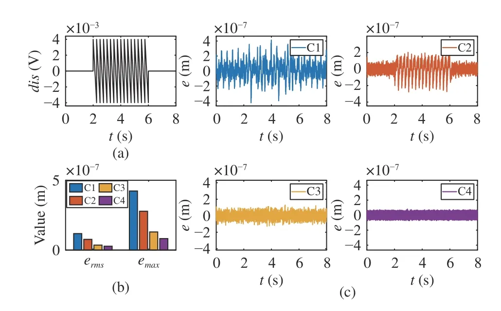
Fig. 6. Simulation results of Disturbance 1 in Case 2, Set 1. (a) Disturbance signal; (b) Performance indexes under different control strategies; (c)Tracking errors under different control strategies.

TABLE II TRACKING PERFORMANCE INDEXES OF CASE 2, SET 1

Since the compensation terms of GRU-NNC and ILC have been determined offline before practical implementation, these two methods are sensitive to accidental disturbances during real-time motion. Consequently, the tracking performance of C1 and C2 significantly deteriorates compared to the condition without disturbances. C3 is an ideal condition which assumes that the accidental disturbance is known in advance.Therefore, ILC can extract the repeated information through several iteration learning trials and suppress the influence of the perturbation as shown in the result of C3. In contrast,ermsandemaxof C4 are 77.73% and 63.24% of C3, respectively.Due to the real-time prediction and compensation process, the RIC method can online adjust the compensation term according to the external disturbance, which results in high tracking accuracy comparable to conditions without disturbance.

• Disturbance 2: Complicated nonlinear signal

Unlike the fixed disturbance signal inDisturbance 1, sometimes the disturbance signal is related to motion parameters such as position and velocity during implementation. Therefore, a complicated nonlinear signal defined as

is added as shown in Fig. 7 (a). Tracking performance of C1−C4 is plotted in Fig. 7 and listed in Table II.

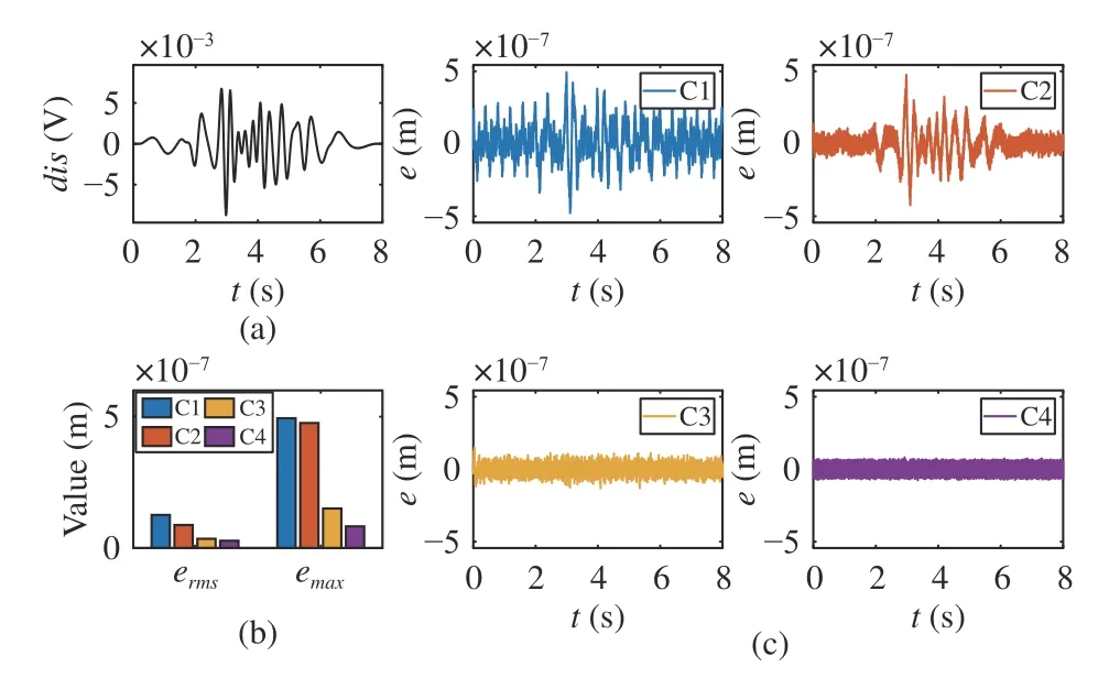
Fig. 7. Simulation results of Disturbance 2 in Case 2, Set 1. (a) Disturbance signal; (b) Performance indexes under different control strategies; (c)Tracking errors under different control strategies.

Similar to the results inDisturbance 1,ermsandemaxof C1 and C2 prominently increase due to the influence of the disturbance signal. For the ideal condition of C3, the tracking performance is still at the same level as Set 1. For the proposed RIC method,ermsandemaxof C4 are 78.37% and 54.65%of C3, which also demonstrates the remarkable disturbance rejection ability of the proposed method. All the simulation results of Case 2 consistently prove that the proposed RIC method can suppress the influence of different forms of uncertain external disturbances.

B. Additional Discussions

The proposed RIC framework is an online trajectory compensation method where both the prediction and compensation processes are completed in one real-time motion control sampling period. In order to verify the real-time implementability, the average execute time of the proposed method during one sampling period is plotted in Fig. 8(a). Obviously,even if the iteration step is set asn=20, the execute time of the RIC method is still far less than the system sampling period. Therefore, the proposed approach satisfies the realtime implementation requirement.

Additionally, Fig. 8(b) illustrates the prediction performance of the established prediction model. For the simple closedloop motion system without any trajectory tracking compensation mechanism applied, the prediction deviation is two orders of magnitude smaller than the actual tracking error.There are almost no reference-induced components in prediction deviations according to the right subfigure of Fig. 8(b).More importantly, the high prediction accuracy can also be achieved with external disturbances injected into the control system. These results validate the excellent prediction accuracy and show that the predicted error is reliable for compensation term generation. Fig. 8(b) also reflect tracking errors of five cases without any feedforward compensation strategies applied. Since the tracking error with compensation is far less than that without compensation, the tracking error under the single PID controller are omitted in Figs. 3−7.

C. Simulation Results of Set 2

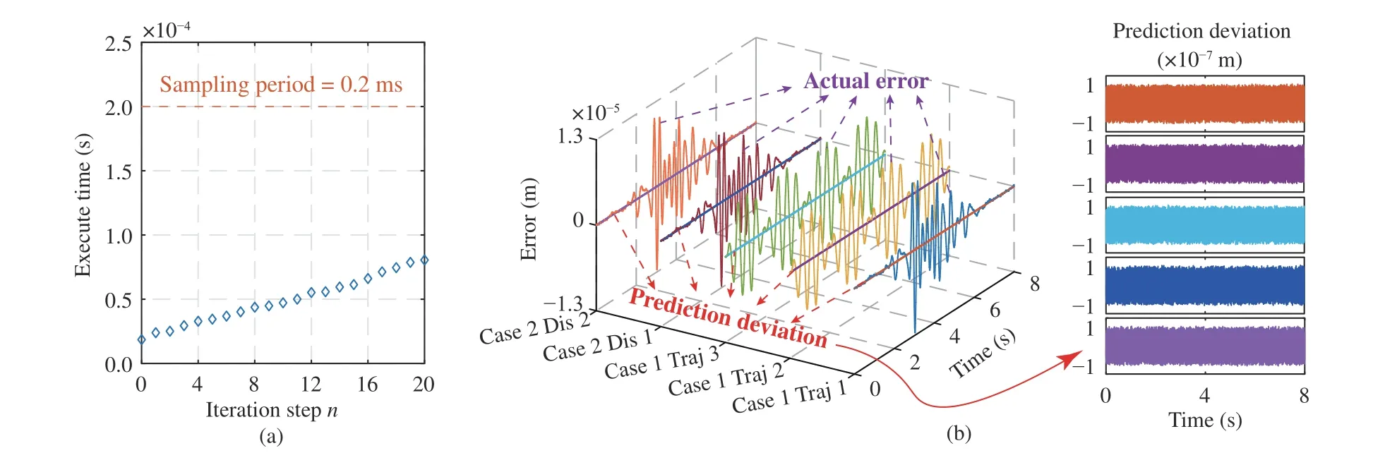
Fig. 8. Additional results of RIC method for Set 1. (a) The relationship between the iteration step n and the average execute time of the proposed real-time algorithm in each motion control sampling period; (b) Prediction accuracy of the proposed prediction model. Here, actual tracking errors and corresponding prediction deviations of five implementations in Set 1 are concurrently plotted in the left subfigure. Since prediction deviations are far less than actual errors,prediction deviations are magnified in the right subfigure for more clear illustration.

To validate the feasibility of the iteration-varying compensation gain when β1does not satisfy the condition (39),another closed-loop transfer function is selected as

whose system parameter β1is identified as β1=2.2046>1.

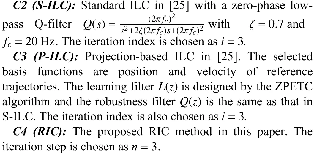
For the proposed RIC method, an iteration-varying compensation gain (52) is designed with the attenuation factor η=2.1>2ln|1/β1|. The simulation motion system is driven to track the NURBS trajectory in Set 1. The tracking performance of the simulation results without external disturbances in this set is plotted in Fig. 9. If the iteration-invariant compensation gain in Set 1 is directly applied to this closed-loop system, the stability and convergence of the entire system cannot be guaranteed since the sufficient condition (39) is not satisfied in this set. As shown in Fig. 9(a), the tracking error will diverge to infinity. In contrast, according toTheorem 2,the iteration-varying compensation gain is available to deal with this defect. The tracking performance under the RIC method with different iteration stepnis shown in Fig. 9(b).Bothermsandemaxwill monotonously decrease as the iteration step increases, and the tracking performance is still comparable to ILC. Additionally, with the same sawtooth wave voltage perturbation in Case 2, Set 1 is added to the control system as an accidental disturbance, the RIC method exhibits its superior disturbance rejection ability compared to ILC as shown in Fig. 10. These results are consistent with the aforementioned results in Set 1. Consequently, the simulation result of Set 2 demonstrates the feasibility of the iterationvarying compensation gain to deal with condition that the condition (39) is unfulfilled.

V. CONCLUSIONS

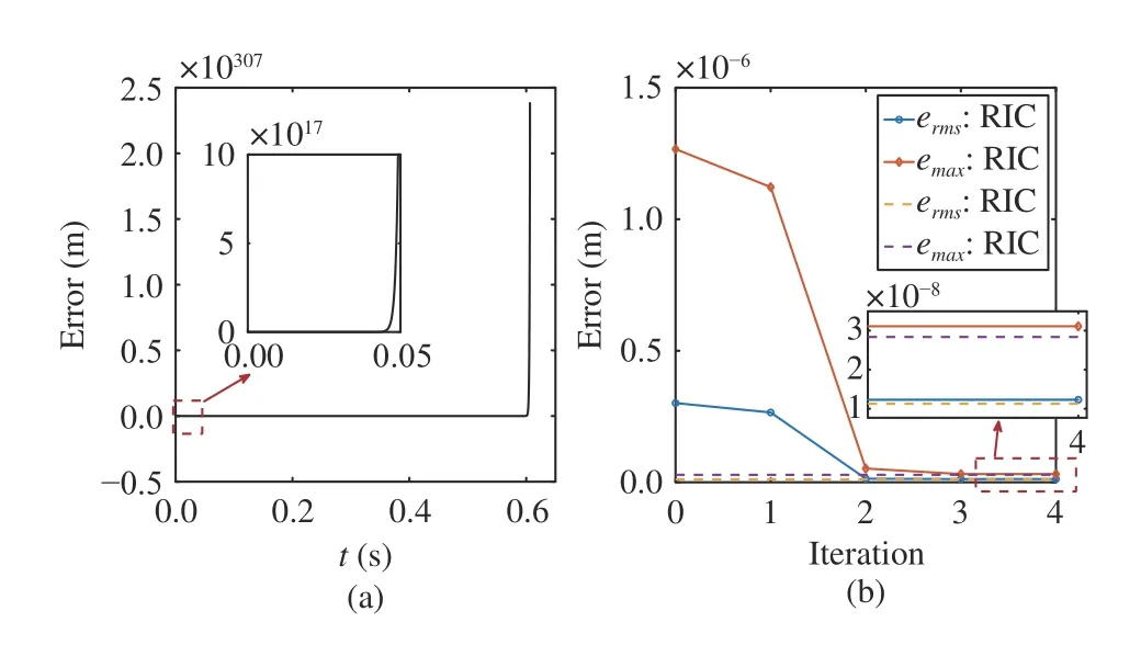
Fig. 9. Simulation results of Set 2 without uncertain external disturbances.(a) Divergence with iteration-invariant compensation gain; (b) Convergence with iteration-varying compensation gain.

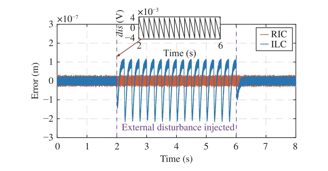
Fig. 10. Simulation results of Set 2 with external disturbances injected.

In this paper, a real-time iterative compensation control framework has been proposed for precision motion systems.An accurate prediction model with external disturbance estimation for a linear SISO closed-looped system is established to predict future tracking errors during real-time motion.On the basis of the predicted errors, an iterative calculation scheme is utilized to generate the corresponding compensation term as a reference trajectory modification. The stability and convergence of the entire control system has been analyzed for different systems to guarantee the feasibility of the proposed method. Superior to offline compensation strategies such as GRU-NNC and ILC, the RIC method omits abundant preimplementations before desired tracking experiments and finishes both prediction and compensation processes in one motion control sampling period. Comparative simulation investigations have sufficiently and consistently proven that RIC not only achieves high tracking accuracy comparable to ILC or even better, but also possesses remarkable robustness to trajectory variations and accidental external disturbances.This strategy is easy to implement since the inner feedback controller structure is unchanged, which makes RIC framework have good potential in mechatronic motion situations.