Characterization of Regional Combustion Efficiency using ΔXCO:ΔXCO2 Observed by a Portable Fourier-Transform Spectrometer at an Urban Site in Beijing※

Ke CHE , Yi LIU , Zhaonan CAI , Dongxu YANG , Haibo WANG ,Denghui JI , Yang YANG, and Pucai WANG

1Key Laboratory of Middle Atmosphere and Global Environment Observation,Institute of Atmospheric Physics,Chinese Academy of Science,Beijing 100029,China

2Carbon Neutrality Research Center,Institute of Atmospheric Physics,Chinese Academy of Science,Beijing 100029,China

3University of Chinese Academy of Science,Beijing 100049,China

ABSTRACT Measurements of column-averaged dry-air mole fractions of carbon dioxide and carbon monoxide, CO2 (XCO2) and CO (XCO), were performed throughout 2019 at an urban site in Beijing using a compact Fourier Transform Spectrometer(FTS) EM27/SUN. This data set is used to assess the characteristics of combustion-related CO2 emissions of urban Beijing by analyzing the correlated daily anomalies of XCO and XCO2 (e.g., ΔXCO and ΔXCO2). The EM27/SUN measurements were calibrated to a 125HR-FTS at the Xianghe station by an extra EM27/SUN instrument transferred between two sites.The ratio of ΔXCO over ΔXCO2 (ΔXCO:ΔXCO2) is used to estimate the combustion efficiency in the Beijing region. A high correlation coefficient (0.86) between ΔXCO and ΔXCO2 is observed. The CO:CO2 emission ratio estimated from inventories is higher than the observed ΔXCO:ΔXCO2 (10.46 ± 0.11 ppb ppm-1) by 42.54%-101.15%, indicating an underestimation in combustion efficiency in the inventories. Daily ΔXCO:ΔXCO2 are influenced by transportation governed by weather conditions, except for days in summer when the correlation is low due to the terrestrial biotic activity.By convolving the column footprint [ppm (μmol m-2 s-1)-1] generated by the Weather Research and Forecasting-XStochastic Time-Inverted Lagrangian Transport models (WRF-X-STILT) with two fossil-fuel emission inventories (the Multi-resolution Emission Inventory for China (MEIC) and the Peking University (PKU) inventory), the observed enhancements of CO2 and CO were used to evaluate the regional emissions. The CO2 emissions appear to be underestimated by 11% and 49% for the MEIC and PKU inventories, respectively, while CO emissions were overestimated by MEIC (30%) and PKU (35%) in the Beijing area.

Key words: FTS,remote sensing,ΔXCO:ΔXCO2,combustion efficiency,megacity

1.Introduction

The increasing anthropogenic emissions of CO2are the main driving force behind global warming induced by greenhouse gases (GHG) (Stocker et al., 2013). Due to increased energy consumption, global fossil CO2emissions reached 9.4 ± 0.5 GtC yr-1over the last decade (2007-17) (Le Quéré et al., 2020). The mitigation of anthropogenic GHG emissions is often accompanied by strengthened air pollution controls (West et al., 2013). The toxic air pollutant CO is an indirect greenhouse gas because it produces positive radiative forcing (0.2 W m-2) through its oxidation reaction with hydroxyl radicals (OH) in the troposphere (Myhre et al.,2013). There was a declining trend of 2% yr-1in CO emissions over East Asia during 2005-16, which mainly resulted from the active clean air policies implemented in China (Zheng et al., 2018a), the largest developing and energy-consuming nation in the world with a very high contribution from megacities.

Urban areas account for 2 % of the world’s land but are responsible for 40%-70% of the global anthropogenic CO2emissions (Satterthwaite, 2008, 2010; Ye et al., 2020). Carbon monoxide (CO) in the urban atmosphere is a product of incomplete combustion alongside the formation of CO2during household combustion, industrial activities, and motor transportation, which results in a general positive correlation between CO and CO2in urban areas. Due to the relatively short lifetime for CO of only a few weeks, it can serve as an unique tracer for atmospheric fossil-fuel CO2emissions and combustion efficiency by analyzing the ratio of CO:CO2.The estimates of combustion efficiency at the urban scale could be calculated from the CO2and CO statistical emission inventories; such an approach is called the “bottom-up”method. Different inventories display significantly different CO2and CO emissions in China, especially at regional and city scales (Zhao et al., 2012; Dai et al., 2020). Accurate measurements of GHG and pollutants in cities are essential to yield significant information about the regional carbon budget and to propose strategies to control these emissions (“topdown ” method). The correlation between CO and CO2could be assessed by directly calculating the slopes of observed CO and CO2volume mixing ratios (Wang et al.,2010; Worden et al., 2012). However, the slopes of CO and CO2are easily affected by annual background growth and biogenic sources. Thus, regression fits of excess CO (ΔCO)and excess CO2(ΔCO2) from continuous observations have been extensively studied to quantify the anthropogenic contribution to carbon variation and source combustion efficiency(Wunch et al., 2009; Silva et al., 2013; Popa et al., 2014;Feng et al., 2019a; Shan et al., 2019; Cai et al., 2021; Park et al., 2021). Megacities in China show a lower combustion efficiency with a higher ΔCO:ΔCO2ratio than in developed countries (Silva et al., 2013; Silva and Arellano, 2017; Park et al., 2021). Studies in Hefei, China have found the Emissions Database for Global Atmospheric Research (EDGAR) and the Peking University (PKU) emission inventories overestimated ΔCO:ΔCO2in central China during 2015-16 (Shan et al., 2019).

Beijing is located in the northern part of China (Fig. 1).It is in a representative fast-growing economic cycle and is a heavily populated and developed region. The air pollution control policies in Beijing are directly related to the country’s overall goals. The total fossil-fuel CO2emissions of Beijing shows high uncertainty with ranges from 1 to 8 Mt in 2012 according to different emission inventories and urban regions (～17% relative to the overall land area of Beijing) contributes about 64% CO2emissions to the total emissions for Beijing (Han et al., 2020). Satellite observations found the XCO:XCO2ratio in Beijing/Tianjin region to be one of the highest in the northern hemisphere due to its rapid economic development (Park et al., 2021). Anthropogenic emissions have been estimated to make a 75.2% contribution to the annual CO2enhancement in Beijing in 2014 based on isotopic analysis (Niu et al., 2016). Long-term,highly accurate in situ measurements of CO2and CO near the surface have been developed in rural and urban regions of Beijing. The Shangdianzi (SDZ) and Miyun sites are used for rural areas, and the Peking University site is used for urban areas (Han et al., 2009; Wang et al., 2010; Feng et al., 2019a; Dayalu et al., 2020). The ratio, ΔCO:ΔCO2, at the Miyun site shows a significant decrease during 2005 to 2008 (Wang et al., 2010). The observation of CO at the SDZ site shows a fast downward trend in 2006-08, is stable in 2009-13, then shows another continuous downward trend after 2013, suggestive of improved combustion efficiencies in response to the Air Pollution Prevention and Control Action Plan implemented in 2013 (Li et al., 2020). The short-term pollution reduction associated with the 2008 summer Olympics and 2020 COVID-19 lockdowns result in a decrease of ΔCO:ΔCO2, suggesting increases in combustion efficiency (Wang et al., 2010; Cai et al., 2021).

The “top-down” analysis of combustion efficiency in Beijing comes mostly from satellite and in situ observations.However, in situ surface monitoring measurements are greatly influenced by vertical mixing. The column-averaged dry-air mole fraction (Xgas) represents the vertically integrated concentration per dry air and is less affected by the vertical motion than in situ measurements. Therefore, the horizontal gradients of Xgashave a more direct relationship with the regional-scale flux (Yang et al., 2007; Wunch et al., 2011;Chen et al., 2016). Satellite observations of XCO2combined with XCO show obvious superiority in global coverage and have been used to quantify the correlation between CO2and CO for Beijing. However, satellite observation is limited by sampling size and temporal resolution to these specific megacities. Satellites make infrequent visits over cities and are easily affected by cloud, aerosol, and topography issues (Lei et al.,2021), leading to insufficient data for urban emissions studies. The Total Carbon Column Observing Network(TCCON) is an international Fourier-transform spectrometer(FTS) network that was originally used for satellite validation and mainly uses ground-based high-resolution Fourier-transform infrared (FTIR) measurements to record information about the GHG column. High-resolution FTIR stations in China have been built at Hefei, Xianghe, and Beijing (Wang et al., 2017; Bi et al., 2018; Yang et al., 2020b). Given the poor transportability of TCCON FTS stations, portable, lowcost FTS is useful as a component in long-term urban column measurements. The EM27/SUN instrument (hereafter,EM27) is a compact FTS with its own solar tracker, which is easy to set up and transport anywhere. FTS measurements in or near urban Beijing have mainly focused on satellite validation (Bi et al., 2018; Yang et al., 2020b). To date, few published studies have rigorously quantified the combustion efficiency in the urban region of Beijing.

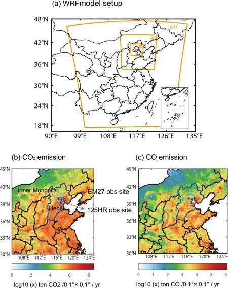
Fig. 1 (a) WRF simulation domains for three grids (27 km, 9 km, 3 km); the red point is the EM27 observation site.The map was taken from a Google satellite image (https://maps.googleapis.com/). Maps of CO2 (b) and CO (c)emissions in 2014 are based on the PKU fossil-fuel emission dataset. Location of the EM27 site (marked by a star) in the center of Beijing (indicated by the closed turquoise line)-Tianjin-Hebei (BTH) area (indicated by the closed blue line) and 125 HR (marked by a star) in Xianghe, Inner Mongolia, Beijing, Tianjin, Hebei are also shown.

In this study, one year of XCO and XCO2measurements based on EM27 were collected at an urban site in Beijing.The objectives of this study were to (1) analyze the correlational relationship between observed enhancements of XCO and XCO2in urban Beijing, (2) reconcile the differences between top-down estimates of combustion efficiency with bottom-up estimates of combustion efficiency, and (3) evaluate the regional CO2and CO emissions estimated from bottom-up inventories using a remote sensing data set. The remainder of this paper is organized as follows. A description of the instrument and method is given in section 2. Section 3 presents the results and discusses their implications and section 4 concludes.

2.Data and methods

2.1.Instrumentation

An EM27 has been set up on the roof of the Institute of Atmospheric Physics (IAP) building in Beijing since 2019.The IAP observation site (highlighted in Fig. 1b) is located between the north 3rd and 4th ring road, with heavy traffic and high CO2and CO emissions. The EM27 spectral resolution is less than 0.5 cm-1, corresponding to a maximum optical path difference of 1.8 cm. The compound InGaAs (indium gallium arsenide) and an extended InGaAs detector are used to stably detect 3800-14 000 cm-1spectral information for accurate column concentrations of CO2and CO (Gisi et al.,2012; Hase et al., 2016). It takes about 60 s to record one individual spectrum with 10 interferograms averaged. The EM27 is equipped with an automated protective case with a rain sensor and a solar irradiation sensor. The cover only opens under cloudless daytime conditions (0000-0900 UTC), protecting the instrument from rain or snow and achieving automated EM27 observations. A WS500 weather station located immediately next to EM27 was used to measure surface temperature and surface pressure with accuracies of 0.2°C and 0.5 hPa, respectively, which were used to correct the a priori temperature profile needed for the XCO2and XCO retrievals. The Bruker OpticalTMInfrared Fourier Transform Spectrometer (IFS) 125 HR used by TCCON is a high-resolution spectrometer(＜ 0.02 cm-1) that is tied to the World Meteorological Organization (WMO) scale through numerous aircraft campaigns(Wunch et al., 2010). To ensure data quality, the EM27 has been calibrated in side-by-side experiments with 125 HR(Gisi et al., 2012; Klappenbach et al., 2015; Hedelius et al.,2017; Frey et al., 2019). High-resolution FTIR stations have been built near Beijing and are located in Xianghe, 50 km east-southeast of Beijing (highlighted in Fig. 1a) (Yang et al., 2020b). The 125 HR at the Xianghe site complies with the TCCON specifications and is used as a calibration reference for the EM27 at Beijing in this study.

A portable EM27 could act as a transfer standard between two FTIR stations (Jacobs et al., 2020). In this study, another EM27 (EM27#2) was used as a mobile transfer standard instrument for 125 HR in Xianghe and the EM27 in Beijing. The EM27#2 took measurements side-by-side with IFS 125 HR during the entire month of November 2019. To ensure stability during the shipment of EM27#2 across Beijing to Xianghe, we examined the ratio between EM27s before and after the shipment. Figures 2a and 2b show the biases between 125 HR and EM27#2. The correction equations are also shown in the figure. Figures 2c and 2d show that the ratio was consistent before and after the shipments (detailed in section 2.2), indicating that the calibration of EM27#2 and 125 HR in Xianghe could be applied to the EM27 retrieval in Beijing. The IFS 125 HR retrievals apply the TCCON standard retrieval code (GGG2014), and the EM27 uses PROFFAST, with the same meteorological data and preliminary profiles input. The results for EM27#2 show a systematic bias with 125 HR, which could be corrected by applying a linear fitting correction function (Figs. 2a and 2b). The biases between EM27 and 125HR are 0.28% and 5.3% for XCO2and XCO, respectively.

2.2.EM27 data processing

A non-linear least-squares fitting retrieval algorithm(PROFFAST) (Hase et al., 2004) is used to analyze the spectra recorded by EM27. The algorithm has been officially used in the EM27 network, COCCON (the COllaborative Carbon Column Observing Network) (Frey et al., 2019). To obtain a high-quality spectrum, the pre-processing steps involve a direct current (DC) correction (Keppel-Aleks et al., 2007), a Norton-Beer medium apodization (Naylor and Tahic, 2007),a fast Fourier transform (Bergland, 1969), and a phase correction (Mertz, 1967). The a priori profiles obtained by TCCON are the official a priori profiles (Toon and Wunch,2015). The inverse algorithm obtains the scaled target gas column by iteratively updating the state variables to best fit the simulated and measured spectra. Finally, the gas column(Cgas) is converted to a dry-air column-averaged mole fraction(denoted Xgas) by dividing the gas column by the simultaneously retrieved column-averaged dry-air mole fractions (Cair)Columnair, where Caircould be calculated from the O2column combined with the volume fraction of O2in the air(20.95%):

In the post-processing process, column averaging kernels(AK) describe the altitude-dependent sensitivity of the retrieved state to the true state. As shown in Fig. 3, AK differs among instruments with different spectral resolutions.EM27 is more sensitive to changes at lower levels than 125 HR, especially for high solar zenith angles (SZAs). A pressure weighting function (PW) is used to weight the pressure thicknesses of each level (ΔP) relative to the surface pressure(Psurf) :

Fig. 2 (a-b) Scatter plots of XCO2 and XCO from 125 HR and EM27#2 side-by-side measurements over the Xianghe Observatory. N is the number of comparison points,B is the bias between the two instruments, R2 is the correlation coefficient, and the equation has the linear fit. (c-d) Scatter plots of EM27 against EM27#2 for different days before and after the EM27#2 transfer calibration campaign. The ratio is the proportional coefficient of EM27(the result for EM27#2 has been taken as a reference).

2.3.WRF -XSTILT model

A Lagrangian particle dispersion model (LPDM) models a plume of atmospheric tracers from a cluster of particles. It can determine the footprint (also called an influence function or adjoint sensitivity) of multiple air parcels released from an observation site (receptor). The WRF-XSTILT, an LPDM model, is adopted to analyze the meteorologicallyinduced gas concentration variation by a regional column footprint simulation ( Lin et al., 2003; Fasoli et al., 2018; Wu et al., 2018). The footprint is used to establish the source-receptor relationship and determine the distribution spread of entire plumes in adjacent cells over the receptor by calculating the sensitivity of the surrounding region (source) to the receptor. The column footprint (Xfoot) is essential for tracking the air masses for column measurements. The parameterXfootis the sensitivity of the column measurements to the upstream and downstream surface-atmosphere fluxes. The formula to calculateXfoot, with units of ppm (μmol (m2s)-1)-1, for each receptor is as follows:

where (xr,tr) is the receptor (r) location, (xi,yi,tm) is the model’s initial time set, denoted by the model grid coordinates of location and time,mairis the mean molar mass of dry air(29 g mol-1),his the atmospheric column height (in XSTILThis set at half the planetary boundary layer (PBL)depth),is the mean density of the air belowh,Nis the total number of released particles, Δtiis the residence time of particle i spent in the grid cell (xi,yi,tm). The total column footprintXfootis the integrated footprint from different vertical altitudes convolved with a pressure weighting function PW(r) and averaging kernel AK(r) at the receptor, which links the emission sensitivity to the observations. In the model setup, we applied the WRF model configurations verified by Dayalu et al. (2020) for the same study domains(Fig. 1a). The receptor site of X-STILT was set up at IAP and was run backward for seven days at a 0.25° × 0.25° spatial resolution to generate hourly column footprints. In each simulation, 100 air parcels are released every 100 m within 3 km and every 500 m from 3 to 6 km relative to the observation level, which tends to be denser near the surface. Higher altitudes are not used since only the lower atmosphere interacts with local emissions in the region (Hedelius et al., 2018).The AK and PW (detailed in section 2.2) of EM27 are used to weight and integrate the footprints of all levels to the column footprint and could be directly obtained from the output of the EM27 retrieval.

Fig. 3 A comparison of the column-averaged kernels at different SZAs for EM27 (a-b) and 125 HR (c-d).

2.4.The ΔXCO:ΔXCO2 calculation method

2.4.1.Calculation ofΔXCO andΔXCO2from measurements

The observed regression slope of ΔXCO against ΔXCO2denotes the amount of CO per CO2emissions in the atmosphere that has been captured by the FTS, signifying the emission ratio or combustion efficiency. A larger slope of the regression line reveals greater combustion efficiency in the observed XCO2. Wunch et al. (2009) proposed that the Xgasanomaly (ΔXgas) could be calculated by subtracting Xgasin the morning from the afternoon value at the same SZA. The anomalies are divided by the AK at the surface to account for the sensitivity of the column measurement to surface variations because diurnal changes are assumed to be confined to the boundary layer. This method could minimize the atmospheric effects from background or natural sources and the SZA-dependent error. The ΔXCO:ΔXCO2ratio, calculated from the diurnal enhancement, is denoted as (ΔXCO:ΔXCO2)d.

Apart from the method based on diurnal variation,ΔXCO and ΔXCO2could be estimated from the regional change relative to the background. The observation site at urban Beijing records the pollution-related signal of XCO and XCO2. The quantification of background XCO2concentration is the sum of the boundary and biogenic XCO2values.

The boundary XCO2value was obtained from trajectory endpoint of the Copernicus Atmosphere Monitoring Service(CAMS) satellite-derived global inversion-optimized mean column concentrations data (http://atmosphere.copernicus.eu/, version: v20r3, last access: 7 June 2021) (Chevallier et al., 2005; Chevallier et al., 2010; Chevallier et al., 2019).These trajectories were derived from the Weather Research and Forecasting-Column Stochastic Time Inverted Lagrangian Transport (WRF-XSTILT). According to the validation report for the CAMS v19r1 data by Chevallier et al.(2020), the biases of modeled XCO2data show less bias(less than 1 ppm) in a non-urban area when compared to the TCCON retrieval results. The background XCO2values obtained from CAMS were mostly from the region less affected by human activities, so the CAMS background values were considered to be plausible. Biogenic XCO2values were from the convolution of the column footprint generated by WRF-XSTILT and the CO2vegetation flux. The CO2vegetation flux comes from a global gridded terrestrial carbon flux product developed by Zeng et al. (2020). Due to unavailable XCO background data, XCO background values were simply obtained from the lowest observed XCO. Similar to the diurnal method described above, the AK at the surface was also taken into account in calculating the anomalies.The ratio ΔXCO:ΔXCO2calculated from regional enhancement is denoted as (ΔXCO:ΔXCO2)r.

2.4.2.Calculation ofΔXCO andΔXCO2from bottom-up inventories

The simulated regression slope of ΔXCO against ΔXCO2represents the regional XCO enhancement per XCO2enhancement contributed from different sources transported to the observation site. A simple way to simulate ΔXCO:ΔXCO2directly from the emission inventories in a specific geometrical shape is as follows (Wunch et al.,2009; Hu et al., 2019; Shan et al., 2019)

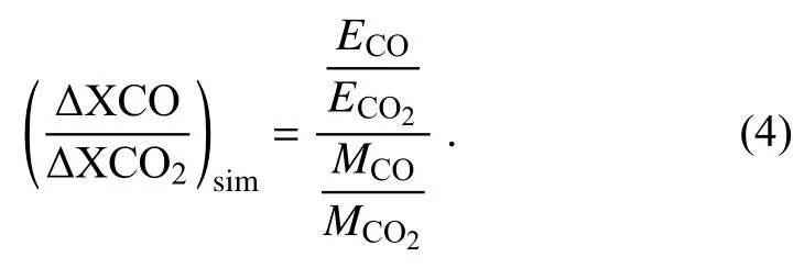
Here,ECOandare the CO and CO2emissions in the s pecific area,andare the molecular masses of CO and CO2, and (ΔXCO/ΔXCO2)simis the simulated correlation slope of XCO to XCO2.

The parameters ΔXCO and ΔXCO2can be simulated by the convolution of the source footprint function (modeled by the Lagrangian atmospheric transport model) and the anthropogenic flux inventories defined as follows:

where the simulated ΔXCO and ΔXCO2are the modeled hourly anthropogenic enhancement from different sources.The(ECO) and is represented by the CO2(CO) surface anthropogenic emissions. The footprint quantifies the sensitivity of the measurements to emissions in terms of unit concentration per unit flux. Simulated ΔXCO and ΔXCO2values based on this method are divided by AK at the surface to account for the sensitivities of column measurements near the surface. We focused on simulations from 1100-1600 local standard time (LST, UTC + 8 h) consistent with the time that the atmosphere is well-mixed and the depth of planetary boundary layer (PBL) grow to approach its maximum in the late morning due to the solar heating of the surface.The PBL, in turn, collapses at sunset due to surface cooling,which increases the difficulty of simulation. We selected this period so that the footprint generated by X-STILT would be less susceptible to modeled PBL uncertainties (Sargent et al., 2018).

3.Results and discussion

3.1.Time series of XCO and XCO2

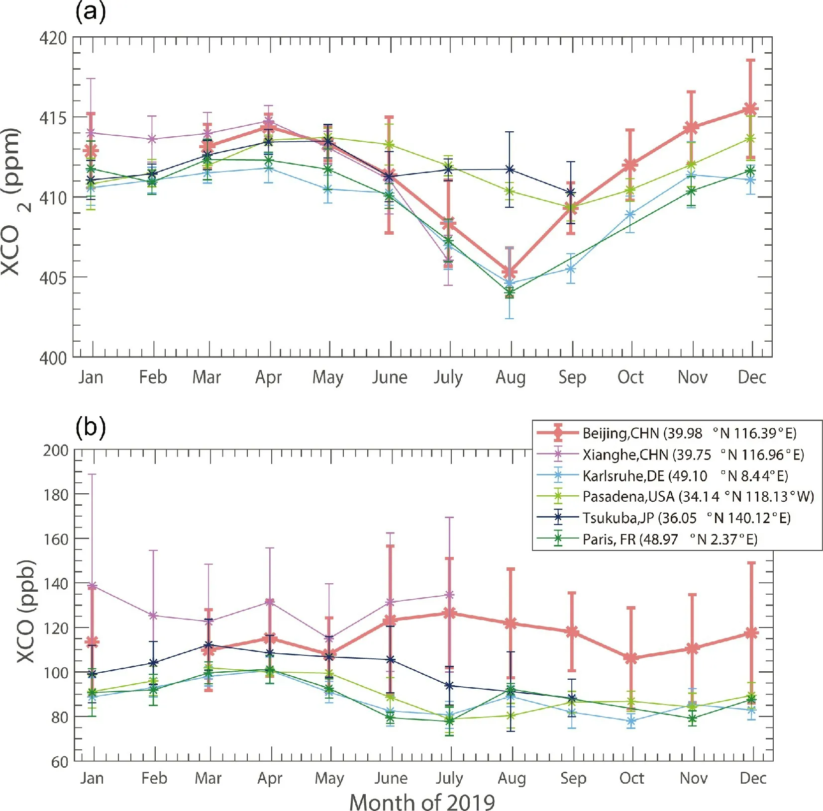
Fig. 4 Monthly variations in (a) XCO2 and (b) XCO observed at Beijing, Xianghe, Karlsruhe, Pasadena,Tsukuba, and Paris during 2019. The geographical coordinates of each site are shown in the figure legend.The error bars are the monthly standard deviation of XCO2 and XCO.

The monthly means and standard deviation of XCO2and XCO at mid-latitude stations in the northern hemisphere are displayed in Fig. 4. These include FTIR stations in Beijing, Pasadena (34.14°N) (Wennberg et al., 2017), Xianghe(39.75°N) (Yang et al., 2020b), Karlsruhe (49.10°N) (Hase et al., 2017), Tsukuba (36.05°N) (Morino et al., 2018), and Paris (48.97°N) (Té et al., 2017). Table 1 summarizes the seasonal mean and standard deviation of XCO2and XCO.There is no data recorded in February, which may cause a bias because anthropogenic XCO2enhancements during the Spring Festival should be significantly lower than normal.The XCO2values in Beijing ranged from 402 ppm to 423 ppm in 2019. The seasonal variation in XCO2achieves its peak in winter (414.33 ± 2.65 ppm), followed by spring(413.58 ± 1.25 ppm) and autumn (412.09 ± 2.88 ppm), and is lowest in summer (407.87 ± 3.34 ppm). The features of the XCO2seasonal variation in Beijing are similar to observations from other FTIR observation sites in the mid-latitude northern hemisphere. Intensity of photosynthesis, which is related to the latitude of the observation site, is the main reason for the seasonality in XCO2variation. The peak and trough of monthly XCO2means were found in December(415.72 ± 3.18 ppm) and August (404.87 ± 1.47 ppm), respectively, which differ slightly from other FTIR stations. The monthly XCO2in Paris, Park Falls, Karlsruhe, and Xianghe stations reach a peak in March to April, whereas Pasadenaand Beijing stations reach a peak in December. The monthly XCO2of Beijing, Xianghe, Paris, Park Falls, Karlsruhe reach a trough in August, whereas Pasadena reaches a trough in September.

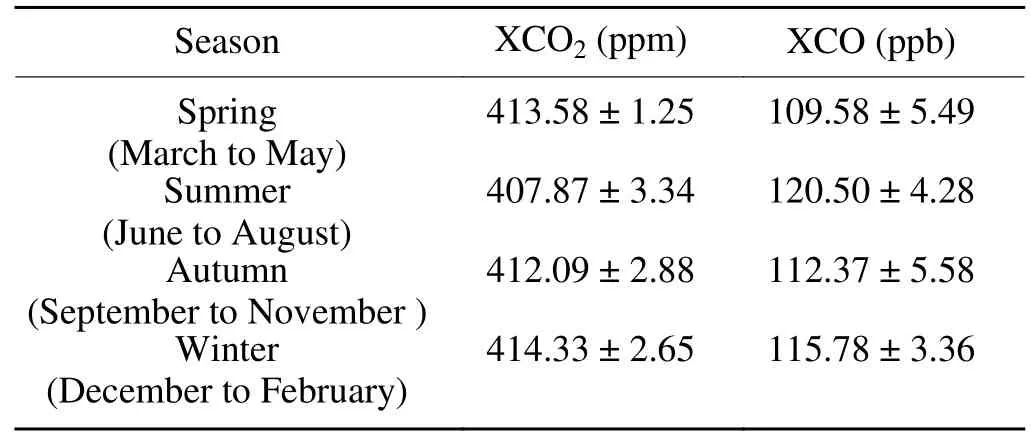
Table 1. Seasonal variability of average XCO2 and XCO in 2019 observed by EM27.

Values of XCO ranging from 85 to 192 ppb are observed in Beijing. The XCO in Beijing was higher than the values from other cities in the northern hemisphere and lower than that of the Xianghe station (Fig. 4b), implying the presence of high regional emissions in the Beijing-Xianghe region. As can be concluded from Table 1,XCO is highest in summer (120.50 ± 4.28 ppb), followed by winter (115.78 ± 3.36 ppb) and autumn (112.37 ± 5.58 ppb),and is lowest in spring (109.58 ± 5.49 ppb). The seasonal variation in Beijing is similar to the variation in Xianghe. The increase of CO during winter in Beijing could be from the increased heating time of vehicle catalysts at low temperatures (Han et al., 2009) and domestic heating. The seasonal variations in Karlsruhe, Pasadena, and Paris show XCO values that are highest in spring and lowest in summer and autumn. The XCO in summer for the Beijing-Xianghe region presents a seasonal variation opposite of the other three urban sites. Carbon monoxide (CO) reaches a minimum during summer at those sites due to strong ultraviolet radiation and high humidity, facilitating the formation of OH, which consumes more CO in the atmosphere (Té et al., 2016; Li et al., 2020). Carbon monoxide (CO) concentration was also found to be lowest in summer from 2006 to 2018 at the Shangdianzi (SDZ) in situ site, a rural region near Beijing (Li et al., 2020). This result is consistent with the Karlsruhe,Pasadena, and Paris sites. The high XCO values in summer observed in urban Beijing and Xianghe could be associated with strong anthropogenic emissions.

3.2.ΔXCO:ΔXCO2 correlation observed by the FTS

Carbon monoxide (CO) is co-emitted and co-transported to the observation site with CO2. The slopes of ΔXCO to ΔXCO2reflect the overall combustion efficiency of the observed airmass. Figure 5 shows the daily regression slope and the Pearson correlation coefficients (R2) of ΔXCO and ΔXCO2based on the diurnal variation method. Daily regression slopes are mostly around 10 ppb ppm-1. Daily correlation coefficients are generally larger than 0.5 on 78% of the observation days. Significant positive correlations between ΔXCO to ΔXCO2in winter, spring, and autumn indicate that most air parcels originate from combustion sources.Approximately 61% of the daily correlation coefficients in summer (grey shaded region in Fig. 5) are small (＜ 0.1) and even negative, and the regression slope shows large uncertainties. This suggests that CO2emissions are dominated by non-CO-related sources in summer. In situ observations near Beijing also captured the low correlation in summer (Wang et al., 2010). The main reason is that the CO2signals were significantly mixed with enhanced biospheric CO2uptake during the growing season, which could offset the anthropogenic emissions in urban areas. It is necessary for CO and CO2to share a common combustion process when using CO as the anthropogenic tracer for CO2to investigate regional combustion efficiency. One straightforward approach is to remove the observations in the growing season (Wang et al., 2010;Shan et al., 2019). Still, we found some strong correlation days in summer (Fig. 5b), so we excluded the non-COrelated observations (R2≤ 0.1). Before filtering the data,(ΔXCO:ΔXCO2)dobserved for urban Beijing is 8.94 ± 0.13 ppb ppm-1with an R2of 0.80. Removal of the strong biologically-affected days contributed to the elevated (ΔXCO:ΔXCO2)dof 10.46 ± 0.11 ppb ppm-1and an R2of 0.86.

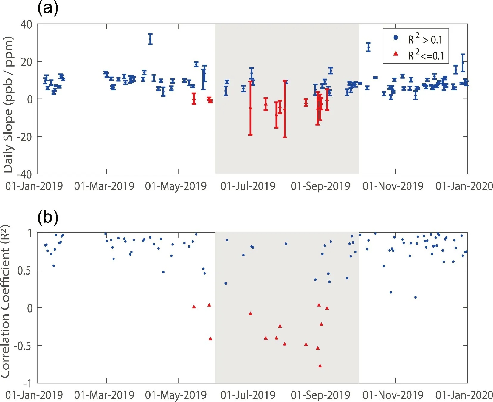
Fig. 5 (a) The time series of the daily slope of ΔXCO and ΔXCO2 observed by EM27 over IAP. The error bar represents the confidence bounds for the slope estimates. (b) The time series of correlation coefficient (R2)of ΔXCO and ΔXCO2. The red triangles represent observations with R2 less than 0.1, and the blue circles represent R2 larger than 0.1. Summertime is indicated by grey shading.

We extended our analysis to comparisons of (ΔXCO:ΔXCO2)dbased on other FTS station datasets of the mid-latitude northern hemisphere in and around 2019 (Table 2).The FTS stations are set up in either an urban or suburban environment with varied emissions sources: the Pasadena site is located on the southern coastal air basin of California with a population of nearly 17 million, the Tsukuba site is located in a highly urbanized city near Tokyo with a population of 2.28 million, the Paris site is in the most populous city in France (2.24 million), the Karlsruhe site is a smaller urban region surrounded by forest, which has a population of nearly 0.3 million. Stronger correlations between ΔXCO and ΔXCO2exist with high regression slope values in the densely populated urban regions (Beijing, Pasadena,Tsukuba, Paris, and Karlsruhe). The values of (ΔXCO:ΔXCO2)dobserved in Chinese cities (10.46 ppb ppm-1in Beijing, 6.76 ppb ppm-1in Xianghe) are significantly higher than stations in other nations. In addition, (ΔXCO:ΔXCO2)din Beijing is the highest among all the cities we included,implying a high pollution per amount of CO2emissions and relatively lower combustion efficiency over Beijing.

According to the in situ observations, Wang et al.(2010) found a ΔCO:ΔCO2value of 41.7 ppb ppm-1at the Miyun background site in Beijing from 2007 to 2008. Han et al. (2009) derived a ΔCO:ΔCO2value of 43.4 ppb ppm-1during the 2006 winter at an urban site in Beijing. Using XCO retrievals from NASA/Terra Measurement of Pollution in the Troposphere (MOPITT) and XCO2retrievals from the Japan Aerospace Exploration Agency Greenhouse gases Observing Satellite (GOSAT), Silva et al. (2013) estimated ΔXCO:ΔXCO2in Beijing/Tianjin to be 43.5 ppb ppm-1from 2009 to 2010. These values are significantly larger than our estimated value (10.46 ppb ppm-1). The reason could be that China has implemented pollution control policies since 2013. As a result, the combustion efficiency significantly increased as CO emissions decreased (Zheng et al.,2018b; Feng et al., 2019b; Li et al., 2020). Shan et al. (2019)estimated ΔCO:ΔCO2to be 15.99, 8.02, and 5.67 ppb ppm-1based on in situ, ground-based FTS, and satellite measurements (GOSAT, MOPITT), respectively, at Hefei from 2015 to 2016. Li et al. (2020) estimated ΔCO:ΔCO2to be 25.5 ppb ppm-1at the SDZ site near Beijing in 2018. The ΔXCO:ΔXCO2value we calculated (10.46 ppb ppm-1) is close to the value estimated from ground-based FTS at Hefei in 2015-16 (8.02 ppb ppm-1) and is about 60% lower than the near-surface observed value at SDZ (25.5 ppb ppm-1). The value of ΔCO:ΔCO2based on FTS (8.02 ppb ppm-1) at Hefei is about 50% lower than in situ observations(15.99 ppb ppm-1) (Shan et al., 2019). In situ observations only capture the near-surface signal of a small sampling area in the local planetary boundary layer. In contrast, the FTS observations detect the whole layer of the atmosphere,which may weaken the near-surface signal. The FTS observations have larger footprint compared to in situ observations and could be more representative to the regional flux(Wunch et al., 2016)

3.3.Effect of regional transportation on ΔXCO:ΔXCO2

Transportation governed by weather conditions plays an important role in the day-to-day variations in CO and CO2in Beijing (Feng et al., 2019a; Panagi et al., 2020). Air pollution is concentrated in Beijing’s southern and eastern parts (Feng et al., 2019a). We identified source regions for each observation based on X-STILT footprints. Pathways are characterized by sources in the northwest (NW) and north China plain (NCP) according to the year-round average 24-hour backward footprints (Figs. 6c and 6e), which share 62.93% and 26.72% of the observation days, respectively.Higher XCO2and XCO occurred when air masses originated from the NCP region. Clean air masses originating from the NW are less affected by human activities, which may cause the observed decrease in XCO2and XCO.

When an air mass passes over different source regions,the correlation between CO and CO2shows different patterns. As shown in Figs. 6b and 6d, (ΔXCO:ΔXCO2)doriginating from the clean region is 8.23 ± 0.1 ppb ppm-1and from the polluted region is 11.46 ± 0.2 ppb ppm-1. Advection that brings air masses containing emissions from the NCP contributed to an elevated proportion of (ΔXCO:ΔXCO2)d,which exceeded the annual slope (10.46 ± 0.11 ppb ppm-1).

Table 2. Comparison of ΔXCO:ΔXCO2 in different FTS stations close or within the urban area in the northern hemisphere.

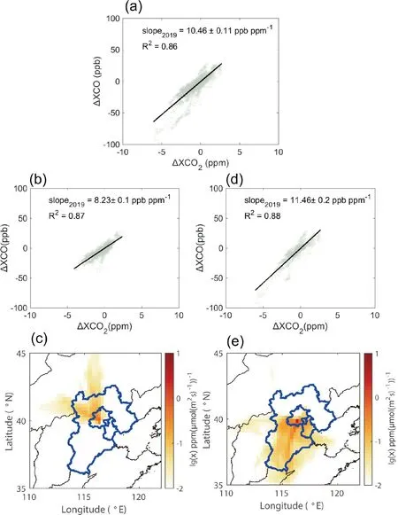
Fig. 6 (a) Correlations of ΔXCO and ΔXCO2 in 2019. (b, d) Correlations of ΔXCO and ΔXCO2 in 2019 originating from the NW and NCP upwind sources. R2 is the correlation coefficient of ΔXCO and ΔXCO2.slope2019 is the regression slope of ΔXCO and ΔXCO2. (c, e) Maps of mean 24-hour backward footprint[ppm / (μmol m-2 s-1), lg(x)] with 0.25° resolution at IAP, Beijing, starting at 1200 LST in 2019, originating from the NW (c) and NCP (e). The closed blue line indicates the BTH area. Only footprint values larger 10-2 ppm / (μmol m-2 s-1) are displayed.

3.4.Comparison of the observed and modeled regional XCO2 and XCO enhancement

The regression slope of ΔXCO:ΔXCO2, based on the regional enhancement method (ΔXCO:ΔXCO2)r, is estimated to be 9.06 ± 1.89 ppb ppm-1, which is consistent with the value of (ΔXCO:ΔXCO2)d(10.46 ± 0.11 ppb ppm-1). The ratio (ΔXCO:ΔXCO2)dis calculated solely based on the diurnal variation observed by EM27. In contrast, (ΔXCO:ΔXCO2)ris estimated by subtracting the background value from the observations. Uncertainty in background value yields more uncertainty for (ΔXCO:ΔXCO2)rcompared to(ΔXCO:ΔXCO2)d.

The estimated values for ΔXCO and ΔXCO2from regional enhancement versus the background were used for comparison with the model simulation at hourly timescales(Figs. 7 and 8). The modeled ΔXCO2(hereafter ΔXCO2,sim)was simulated from the MEIC and PKU anthropogenic emission inventories (ΔXCO2,MEICand ΔXCO2,PKU). The observed enhancement ΔXCO2(hereafter ΔXCO2,obs) was the difference between the observed urban XCO2(XCO2,obs)and the XCO2background (XCO2,back) from model. Summer data is excluded due to the unavailable background data for CO (detailed in the next paragraph). The same trend is shared by XCO2,backand XCO2,obsas shown in Fig. 7a.

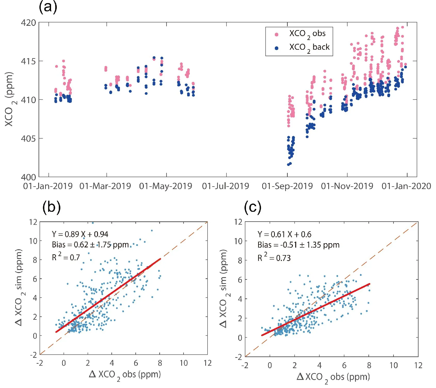
Fig. 7 (a) Measured XCO2 and CAMS background concentration. (Only 1100 to 1600 LST periods are displayed). (b-c) Hourly measured and modeled regional enhancement ΔXCO2 for each fossil-fuel emission inventory (b for MEIC, c for PKU).

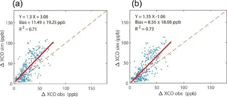
Fig. 8 Hourly measured and modeled XCO for (a) MEIC and (b) PKU.

Figures 7b and 7c show the correlation between ΔXCO2,obsand ΔXCO2,sim. The x-intercept of the linear fitting equation of (～1 ppm for MEIC and PKU) represents the ΔXCO2,obsvalue with no anthropogenic effect. The bias of ΔXCO2,obsand ΔXCO2,simwas mainly attributed to the error from emission inventories, background XCO2values, and transport simulation. Both the observed and modeled ΔXCO2are in good agreement, with correlation coefficients(R2) of 0.70 and 0.73 for MEIC and PKU, respectively. The slope of the fitting equation denotes the ratio of the observed ΔXCO2change to the modeled ΔXCO2change.Many previous studies attempted to use the slope value as a scale factor to evaluate and constrain regional CO2emissions(Sargent et al., 2018; Shekhar et al., 2020; Yang et al.,2020a). The slope for MEIC (0.89 ppm ppm-1) is closer to the 1:1 line than PKU (0.61 ppm ppm-1). According to the regression slope value, MEIC underestimates approximately 11% of CO2emissions surrounding Beijing and PKU underestimates approximately 49%.

Figure 8 denotes the correlation plots of observed ΔXCO (ΔXCOobs) and modeled ΔXCO (ΔXCOsim). The ΔXCOobsdata is correlated to ΔXCOsimwith R2of 0.71 and 0.73 for MEIC and PKU, respectively. The minimum of the observed XCO (80.0 ppb) was taken as a constant XCO background value. The x-intercepts for MEIC (77.63 ppb) and PKU (80.79 ppb) show consistency and agree with the minimum of observed XCO. However, the constant background value could not capture the variation of the true XCO background, especially for summer with strong biological-influenced (detailed in section 3.1). Therefore, the ΔXCO data in Summer are excluded. The slopes for MEIC (1.3 ppb ppb-1)and PKU (1.35 ppb ppb-1) indicate an overestimation of approximately 30% and 35%, respectively, for CO emissions surrounding Beijing.

3.5.Comparison the observed and simulated ΔXCO:ΔXCO2

Many studies have compared the observed ΔCO:ΔCO2with emission inventories (Turnbull et al., 2011; Tohjima et al., 2014; Shan et al., 2019). To calculate the simulated ΔCO:ΔCO2with emission inventories on a regional scale, it is essential to know that the observational site is representative of the region. A few studies roughly specified a geometric bounding box outlining the region which influences the observed value (Wunch et al., 2009; Hu et al., 2019; Shan et al., 2019). However, ΔCO:ΔCO2calculated based on the geometric bounding method is sensitive to the specified size of the enclosed area. A circle centered upon the EM27 observation site was specified as the influencing region. As the source area radius ranges from 50 to 500 km, ΔCO:ΔCO2varies from 17.00 to 19.77 ppb ppm-1for MEIC, 32.28 to 53.74 ppb ppm-1for PKU, respectively. The results show great uncertainty among different inventories and influencing areas. This method is based on the assumption that each grid in the specific geometric region of the emission map contributes equally to the observed concentration.

The region of influence and the sensitivity of each influencing grid to the observations vary over time. Using surface hourly backward column footprints for each measurement is a common and robust way to quantify the sensitivity of the atmospheric concentration changes at the receptor to upwind source regions using units of concentration per unit flux (Turnbull et al., 2011; Tohjima et al., 2014). Each footprint is convolved with the corresponding hourly gridded emission inventories (PKU, MEIC). The modeled anthropogenic enhancement of CO and CO2at the receptor site is the sum of contributions from the sensitive emission grid flux (detailed in section 2.3). The linear regression slopes of the modeled ΔXCO:ΔXCO2based on PKU, MEIC, and observations are shown in Table 3. The outliers are excluded according to the three standard deviations criterion. Modeled ΔXCO shows a good relationship with ΔXCO2with R2of 0.97 for MEIC and 0.96 for PKU. The modeled data displays a slightly greater correlation than the observed ΔXCO and ΔXCO2(R2= 0.86 for the diurnal variation method, R2=0.83 for the regional enhancement method). The reason is that modeled values only take the anthropogenic influence of CO into account, ignoring the CO2-related but not the COrelated signal, such as the resident respiration of CO2. The observed ΔXCO and ΔXCO2values based on regional background enhancement display the weakest correlation (R2=0.83) due to the uncertainty of the modeled background value. The simulated regression slope of ΔXCO and ΔXCO2in 2019 is 14.91 ± 0.36 ppb ppm-1for MEIC and 21.04 ± 0.70 ppb ppm-1for PKU. The MEIC and PKU inventories are 42.54% and 101.15% higher than the observed value (10.46 ± 0.11 ppb ppm-1), respectively.

In recent studies, ΔXCO:ΔXCO2based on EDGAR(PKU) emission inventories are about 256.59% (219.39%)larger than the values calculated from the FTS in Hefei 2015-16, and 207.86% (173.31%) larger than those in 2016-17 (Shan et al., 2019). Silva and Arellano (2017)found that ΔCO:ΔCO2based on the EDGAR inventory was 50% higher than the value estimated by satellites in the megacities of China. Wang et al. (2010) found that the bottom-up estimate of ΔCO:ΔCO2was 19.2% larger than theobservations at Miyun, Beijing, during winter 2006. Despite the observation and comparative methods, the emission inventories in urban China might overestimate ΔCO:ΔCO2. The lack of consideration of CO2emissions from the respiration of the residents in dense urban regions may lead to the overestimation of bottom-up-based ΔCO:ΔCO2(Wang et al.,2010). Either the overestimation of CO anthropogenic flux or under-consideration of CO sinks are possible reasons for the elevated bottom-up estimates of ΔCO:ΔCO2(Vardag et al., 2015; Shan et al., 2019).

Table 3. Comparison of the observed and simulated ΔXCO:ΔXCO2.

The main reason why MEIC and PKU overestimated ΔXCO:ΔXCO2surrounding Beijing is likely due to the overestimation of the regional CO emissions and underestimation of CO2emission. The ΔXCO and ΔXCO2discussed in section 3.4 are directly linked to the regional emission. The difference between the modeled and observed ΔXgasis directly proportional to the difference between the emission inventories and the actual emission. The deviation of the regression fitting equation with the 1:1 line shows the model-observed difference. The slope value of modeled ΔXCO to observed is less than one, suggestive of typical overestimations of CO emissions of 30% and 35% for MEIC and PKU, respectively.The underestimation of CO2emissions magnifies the effects of overestimated CO emission, which contributes to the larger difference between the modeled ΔXCO:ΔXCO2and the observed ratio. For MEIC, a relatively smaller underestimation of CO2emissions makes the modeled ΔXCO:ΔXCO2closer to observations.

4.Conclusions

Data was collected for clear days over one year for XCO and XCO2using the portable FTS EM27 in the urban area of metropolitan Beijing. The overall variation in XCO2typical variations in anthropogenic emissions (traced by the XCO variation) which are overlaid upon the biogenic and meteorological field effects. Correlation analyses between the XCO and XCO2enhancements provided useful information to identify the characteristic of combustion efficiency in Beijing. The (ΔXCO:ΔXCO2)dobserved in urban Beijing(10.46 ± 0.11 ppb ppm-1) is higher than other FTS urban stations (Karlsruhe, Pasadena, Tsukuba, and Paris), suggesting a high anthropogenic proportion of CO2emissions and lower combustion efficiency in Beijing. Daily ΔXCO:ΔXCO2varies remarkably with seasonality and weather conditions. The ΔXCO:ΔXCO2in summer shows large uncertainty, and the correlation of ΔXCO and ΔXCO2is weaker than the other three seasons. According to the air mass pathways arriving in Beijing tracked by the WRF-XSTILT model, the observation site had upwind sources from the NW and NCP of 62.93% and 26.72% of overall observation days, respectively. Air masses passing over the NCP region increased the proportion of ΔXCO to ΔXCO2(11.46 ± 0.20 ppb ppm-1), which exceeded the slope with a clean upwind source (8.23 ± 0.10 ppb ppm-1). When backward column footprints were combined with emission inventories, observations could be quantitatively compared with the emission inventories. The MEIC and PKU inventories are 42.54% and 101.15% higher than the observed values, respectively.After comparing the observed regional enhancement with the modeled ΔXCO and ΔXCO2, the main reason for the difference is the overestimation of the regional CO emissions and underestimation of CO2emission. The less drastic underestimation of CO2emissions for the MEIC results in the improved modeling of ΔXCO:ΔXCO2compared to PKU.This work highlights the necessity for long-term column measurements in the heavily CO-emitting Beijing region. However, one station could only capture limited information on a regional scale within a larger urban signal. The background value obtained from the model contains a degree of uncertainty. Compared to in situ surface observations, FTS stations only record the Xgasin clear-sky days, which can potentially lead to bias from a less homogeneous sampling. An intensive experimental FTS station combined with WRF-XSTILT could open up additional potential pathways for regional emissions studies.

Acknowledgements.We want to thank the TCCON community for providing the FTIR observations of Pasadena, Karlsruhe,Tsukuba, and Paris. This study is supported by grants from the National Key Research and Development Program of China (Grant No. 2017YFB0504000), National Natural Science Foundation of China (Grant No. 41875043), the Strategic Priority Research 275 Program of the Chinese Academy of Sciences (Grant No.XDA17010102), External Cooperation Program of the Chinese Academy of Science (Grant No. GJHZ1802), Youth Innovation Promotion Association, CAS.