One-Dimensional Variational Retrieval of Temperature and Humidity Profiles from the FY4A GIIRS
Qiumeng XUE, Li GUAN*, and Xiaoning SHI
1Collaborative Innovation Center on Forecast and Evaluation of Meteorological Disasters, Key Laboratory for Aerosol-Cloud-Precipitation of China Meteorological Administration, Nanjing University of Information Science and Technology, Nanjing 210044, China
2Department of Mathematics, University of Wisconsin-Madison, Madison 53706, USA
ABSTRACT A physical retrieval approach based on the one-dimensional variational (1D-Var) algorithm is applied in this paper to simultaneously retrieve atmospheric temperature and humidity profiles under both clear-sky and partly cloudy conditions from FY-4A GIIRS (geostationary interferometric infrared sounder) observations. Radiosonde observations from upper-air stations in China and level-2 operational products from the Chinese National Satellite Meteorological Center (NSMC)during the periods from December 2019 to January 2020 (winter) and from July 2020 to August 2020 (summer) are used to validate the accuracies of the retrieved temperature and humidity profiles. Comparing the 1D-Var-retrieved profiles to radiosonde data, the accuracy of the temperature retrievals at each vertical level of the troposphere is characterized by a root mean square error (RMSE) within 2 K, except for at the bottom level of the atmosphere under clear conditions. The RMSE increases slightly for the higher atmospheric layers, owing to the lack of temperature sounding channels there.Under partly cloudy conditions, the temperature at each vertical level can be obtained, while the level-2 operational products obtain values only at altitudes above the cloud top. In addition, the accuracy of the retrieved temperature profiles is greatly improved compared with the accuracies of the operational products. For the humidity retrievals, the mean RMSEs in the troposphere in winter and summer are both within 2 g kg-1. Moreover, the retrievals performed better compared with the ERA5 reanalysis data between 800 hPa and 300 hPa both in summer and winter in terms of RMSE.
Key words: temperature and humidity profiles, one-dimensional variational (1D-Var), GIIRS, hyperspectral data
1. Introduction
Atmospheric temperature and humidity profiles are essential to climate research. Continuous and frequent atmospheric temperature and humidity profiles are of great significance for improving the accuracy of nowcasting applications and situational awareness. Atmospheric temperature and humidity profiles from conventional radiosonde data have high representativeness and dependability. However, due to their low temporal and spatial resolutions, it is difficult for radiosonde measurements to meet the requirements for global climate and weather model development. To solve this problem, satellite-based hyperspectral infrared (IR)sounders have been developed in recent decades due to their unique advantages (Menzel et al., 2018). Hyperspectral infrared sounders onboard meteorological satellites can monitor vertical temperature and humidity structures on a global scale with a high temporal resolution (Yang et al., 2017). In addition, hyperspectral infrared sounders have thousands of channels with high vertical resolution, which can display more detailed and accurate vertical profiles of atmospheric temperature and humidity (Strow et al., 2003; Pougatchev et al., 2009).
Temperature and humidity profiles can be obtained from hyperspectral infrared sounder measurements by combining the IR radiation transmission model with a retrieval algorithm. Much work so far has focused on these retrieval algorithms. King (1956) first proposed the concept of using radiation received by infrared sounders to retrieve atmospheric temperature. Kaplan (1959) reported that atmospheric temperatures at different heights can be retrieved by using radiation from different spectral regions originating from different atmospheric layers. More recently, the main retrieval methods are generally divided into three types: statistical approaches, machine learning approaches, and physical approaches. The statistical regression approach depends on the regression equation established by the atmospheric parameters and the satellite measurements from the spectral channels. This method does not consider the physical characteristics of atmospheric radiation transmission and cannot describe the important nonlinearities between geophysical variables and radiances. Therefore, in this method, the accuracy of the retrievals is determined by the temporal and spatial representations of the statistical samples. Even so, this method has advantages due to the efficiency of its calculations. Several scientists have described the eigenvector statistical method. Smith and Woolf (1976) illustrated a statistical regression approach to retrieve atmospheric parameters from measured radiance values using eigenvector covariance matrices. Guan (2006) retrieved atmospheric temperature and humidity profiles and surface skin temperature from atmospheric infrared sounder (AIRS) observations with an eigenvector statistical technique based on principal component analysis. Jiang et al. (2006) implied that temperature and humidity profiles retrieved from AIRS by using eigenvector covariance matrices can meet the basic requirements of atmospheric profile retrieval accuracy: 1 K for temperature and 20% for relative humidity in 1 km-thick tropospheric layers. The use of the eigenvector statistical method for retrieving temperature and humidity profiles from AIRS has also been performed by many other scholars (Liu et al.,2008; Smith et al., 2012; Zhang et al., 2014). Other statistical regression methods, including the ridge regression method (Xi and Wang, 1984), the cumulative sum statistical control method (Zhang and Wang, 1995), the empirical orthogonal function method (Han et al., 2009), and the least-squares method (Xu, 2003), have been widely used to retrieve atmospheric profiles. In recent years, machine learning algorithms have been gradually introduced into the field of atmospheric science. Yao and Chen (2006) demonstrated that the overall root mean square errors of profiles retrieved by the neural network method are 17% lower over the ocean and 15% lower over land compared to those obtained by using the statistical retrieval method. Singh and Bhatia(2006) retrieved real-time atmospheric temperature and humidity profiles by using a neural network based on the advanced microwave sounding unit (AMSU) over the Indian region and reported that the retrieved temperature and humidity profiles were in good agreement with the measurements from the AIRS, with a notable biased warming and moistening under 850 hPa, of 3 K and 4 g kg-1. Paola et al. (2018) created temperature and water vapor profiles using the random forest technique (MiRTaW) based on observations from the advanced technology microwave sounder(ATMS). Malmgren-Hansen et al. (2019) were the first to present a convolutional neural network used for the retrieval of atmospheric profiles from the Infrared Atmospheric Sounding Interferometer (IASI) sounding data and observed large gains in retrieval accuracy when predicting profiles over clouds.
As mentioned above, the statistical approach is dependent on a large training dataset, and the physical nature of atmospheric radiation transmission is not considered, which affects the accuracy of the retrievals. The physical approach aims to retrieve atmospheric temperature and humidity profiles directly from satellite measurements of spectral channel radiation. This approach solely takes atmospheric radiation transmission into account and has no dependence on training samples. Physical methods require prior statistical information and involve radiative transfer calculations and iterative solutions (Duncan and Kummerow, 2016). Many methodologies have been proposed to estimate these iterative solutions (Chahine, 1970; Smith, 1970; McMillin,1991). Among those methodologies, the variational method lays a foundation for retrieving atmospheric parameters from IR hyperspectral and microwave sounder measurements. Li et al. (2000) retrieved temperature profiles through Newton nonlinear iteration based on the 1D-Var principle from the International Advanced Television and Infrared Observation Satellite Operational Vertical Sounder(ATOVS) and the retrieval accuracy is about 2 K at 1 km vertical resolution. Susskind et al. (2003) described the basic methodology, based on the variational method used by the AIRS Science Team, to analyze AIRS data in the presence of clouds and determine atmospheric temperature and humidity profiles. Wu et al. (2005) reported that the root mean square errors of profiles retrieved from AIRS clear-sky measurements over 850 hPa were less than 1 K for temperature profiles and 10% for humidity profiles. Recently, many investigators have widely used the 1D-Var algorithm to retrieve atmospheric parameters and have developed assimilation systems for a variety of microwave sensors, infrared hyperspectral sounders, and ground-based microwave radiometers (Li and Zeng, 1997a, 1997b. Liu and Weng, 2005; Martinet et al., 2017).
A new generation of Chinese geostationary meteorological satellites called Fengyun-4A (FY-4A) was successfully launched into space in 2016. The Geostationary Interferometric Infrared Sounder (GIIRS) onboard FY-4A is the first infrared hyperspectral sounder onboard a geostationary weather satellite with greatly enhanced capabilities for highimpact weather event monitoring, warning, and forecasting.He et al. (2019) reported that temperature profiles are available only at altitudes above the cloud top, and humidity profiles are not provided in the present operational products released by the Chinese National Satellite Meteorological Center (NSMC). Nearly half of the level-2 operational atmospheric temperature and humidity products from the NSMC are labeled perfect, even in clear-sky conditions; under cloudy sky conditions, only 30% of the products are categorized as perfect, according to the quality flag suggested by the Fengyun science team. It is therefore desirable to improve the accuracy and increase the number of the profiles retrieved based on GIIRS observations. In this paper,the 1D-Var physical retrieval algorithm is applied to hyperspectral infrared GIIRS data to retrieve atmospheric temperature and humidity profiles under both clear-sky and partly cloudy conditions. At the same time, radiosonde data are used to validate the performances of the FY4A operational products from the NSMC and of the profiles retrieved in this study.
The remainder of this paper is organized as follows. Section 2 describes the data and the model used, section 3 discusses the retrieval methodology, section 4 presents the results and provides for a discussion, and section 5 concludes.
2. Data and model
2.1. GIIRS data
FY-4 series comprises China's second-generation geostationary meteorological satellites. As the first flight unit of the FY-4 series, FY-4A was successfully launched into space on 11 December 2016, carrying the Advanced Geosynchronous Radiation Imager (AGRI), Geostationary Interferometric Infrared Sounder (GIIRS), and the Lightning Mapping Imager (LMI) (Yang et al., 2017). FY-4A’s GIIRS is the first high-spectral-resolution advanced IR sounder onboard a geostationary weather satellite, complementing the advanced IR sounders in polar orbit and providing nearly continuous temporal, horizontal, and vertical observations.
The GIIRS is a Michelson Fourier transform infrared interferometer that measures atmospheric infrared radiation,covering the range of the long-wavelength IR (LWIR) band(700-1130 cm-1) and the mid-wavelength IR (MWIR) band(1650-2250 cm-1) at a spectral resolution of 0.625 cm-1. It has 1650 spectral channels, of which 689 channels are for the LWIR band and 961 channels are for the MWIR band.As FY-4A moves, the GIIRS observes a total of 128 fields of view (FOVs) arranged in a 32 × 4 array, corresponding to an FOV with a 16-km diameter at nadir. The specific GIIRS instrument characteristics are given in Table 1 (Yu et al.,2020).
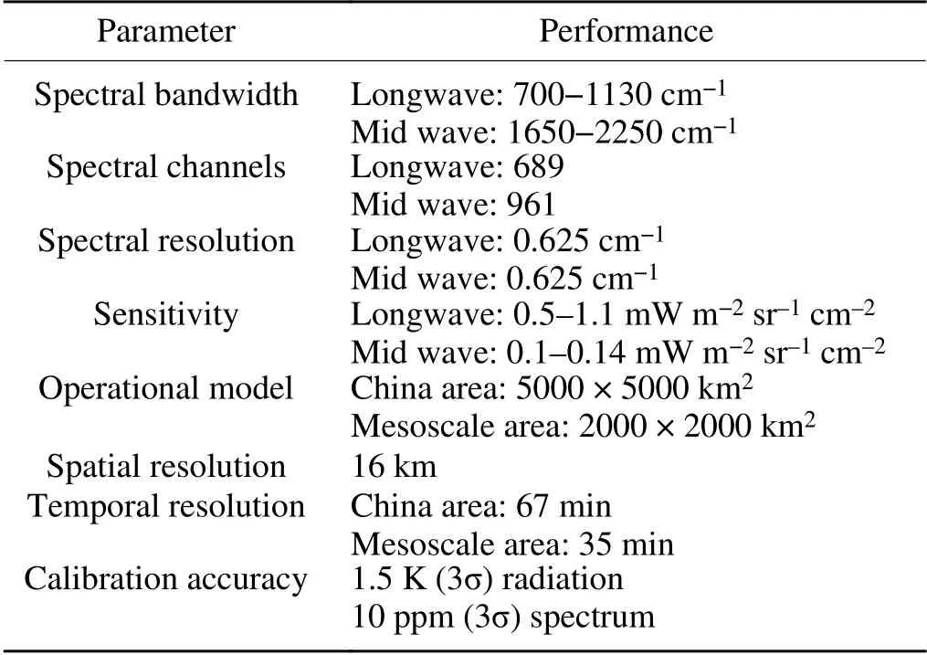
Table 1. Specification for GIIRS onboard FY-4A.
In this study, GIIRS level-1 (L1) observed data and level-2 (L2) operational products from December 2019 to January 2020 (winter season) and from July 2020 to August 2020 (summer season) were collected twice daily, at 0000 to 0100 and 1200 to 1300 Coordinated Universal Time(UTC). The GIIRS L1 observed data can provide information such as the measured radiation values of the 1650 channels, noise equivalent spectral radiation values, and the longit-ude and latitude of the observation points. The GIIRS L2 operational products include the temperature profile of the GIIRS, cloud mask, land/sea mask, and surface parameters.The GIIRS L1 and L2 datasets can both be downloaded from the Chinese National Satellite Meteorological Center(NSMC).
2.2. Radiosonde data
The radiosonde data of specific synoptic hours from upper-air stations in China are used to estimate the performance of both the retrieved profiles and the GIIRS profile products from the NSMC. The radiosonde data are received twice daily, at 0000 and 1200 UTC, from the China Meteorological Data Service Center (CMDC). Sounding observations from December 2019 to January 2020 and from July 2020 to August 2020 from 89 upper-air stations in the China area were used in this paper. The data include observational information such as geopotential height, temperature,dew point temperature, wind direction, wind speed at all specific isobaric levels, and pressure-temperature-humidity layers.
2.3. ERA5 data
In 2018, the European Centre for Medium-Range Weather Forecasts (ECMWF) released its fifth-generation global climate reanalysis dataset, called ERA5, which is produced using 4D-Var data assimilation in CY41R2 of ECMWF’s Integrated Forecast System (IFS), with 137 hybrid sigma/pressure (model) vertical levels, with the toplevel at 0.01 hPa. Atmospheric data are available on these levels and are also interpolated to 37 pressure, 16 potential temperature and 1 potential vorticity level(s). The ERA5 dataset has a horizontal resolution of 0.25° × 0.25° (± 31 km at the equator) and a temporal resolution of 1 h (Hersbach et al., 2020). In this paper, atmospheric parameters at 37 pressure levels, including temperature, specific humidity, and ozone mass mixing ratio, were collected at 0000 to 0100 UTC and again at 1200 to 1300 UTC as initial guesses for the 1D-Var retrieval. Surface level parameters, including surface pressure, geopotential, and skin temperature, were used at the same time. To address the pressure level mismatch, a regression matrix was applied to map the data from the ERA5 37 pressure levels to the 101 levels required by the retrieval, which is consistent with the levels of the U.S. standard profile.
2.4. Forward model
The forward model is one of the most critical components of the retrieval algorithm. It computes radiances in a clear-sky corresponding to given atmospheric and surface states as well as Jacobian radiances with respect to atmospheric and surface parameters for use by the retrieval module. In this study, the Community Radiative Transfer Model(CRTM) developed by the United States Joint Center for Satellite Data Assimilation (Weng et al., 2005) was applied.In the 1D-Var retrieval algorithm, the initial profiles generated from the ERA5 datasets were used as inputs for CRTM. The number of levels in the CRTM model was set to 101, which is consistent with the input profiles for the retrievals.
3. Introduction of retrieval methodology
3.1. Theoretical basis of the 1D-VAR retrieval algorithm
The retrieval methodologies adopted for both microwave and infrared radiation are essentially based on finding the solutions by minimizing a cost function of the following form (Rodgers, 1976):

where y and F(x) represent the observed radiances and the radiances calculated by the forward model and x is the atmospheric state vector. If both the state vector and the radiances are characterized by Gaussian distributions, then the cost function can be minimized by the following form:

where B and O represent the background error covariance matrix and observation error covariance matrix describing the measurement, respectively; xbis the background state vector, namely, an a priori vector; F(x) is the radiance simulated using the forward model, and y is the observed radiance. The first term in Eq. (2) on the right represents the cost function on the right represents the penalty for departing from the a priori information, while the second term represents the penalty for departing from the measurements.The algorithms used to minimize the cost function include the linear iterative method, the Gauss-Newton nonlinear iterative method, the steepest descent method, and the Levenberg-Marquardt method. In this study, the Newton method was adopted to seek the iterative solution to the inversion problem by minimizing this cost function (Martinet et al.,2015). When the term with y-F(x) in the second partial derivative is neglected (Li and Zeng, 1997a), the final onedimensional variational iteration equation can be written as follows:

where n is the iteration number; xnand xn+1represent the profiles of atmospheric temperature and humidity at steps n and n+1 in the iteration process, respectively; and K is the Jacobian matrix containing partial derivatives of y with respect to x, as calculated by the forward model. The NMC method was utilized to compute the background error covariance matrix from the differences between the 48-hour and 24-hour forecasts provided by the ECMWF operational forecasts.The set of forecast differences consists of two daily runs(starting at 0000 and 1200 UTC) over two, two-month periods which include December 2019 and January 2020, and July and August 2020. To further handle the nonlinearity of the retrieval problem, the DRAD approach is used in the above Newtonian method to ensure that the retrieval is stable (Lynch et al., 2009). In the DRAD approach, the diagonal element of the observation error covariance matrix, O,is set to either the difference between the observed and simulated radiances for a particular spectral channel or to the instrument noise plus forward model error:

where α is the configurable error parameter, which is set to 2 in this paper and σ(j) is the instrument noise variance for channel j. The role of α is to limit the magnitude of xn+1-xnat each iteration step. As the number of iterations increases, the difference term quickly vanishes, and the final solution is obtained. Finally, a chi-square test is used to check the convergence of the retrieval (Divakarla et al.,2014). The chi-square test acts as a gauge of the consistency between the radiances calculated by the forward model and the observed GIIRS radiances relative to instrument noise errors. The equation is as follows:

where n chan is the number of channels used in the retrieval and ysim,jis the simulated radiance using the forward model.The termination criteria of the iteration require χ2to be less than 0.7 or an iteration number greater than 9.
3.2. GIIRS data matching
To generate the initial guess profiles, it is necessary to collocate the ERA5 datasets with the GIIRS observational field of view by temporal-spatial matching. The first step in the matching process is the spatial interpolation of the ERA5 data on a standard grid to the latitude and longitude of the GIIRS FOV using a bilinear interpolation. The second step is the temporal interpolation of the ERA5 data to the GIIRS observational time. The ERA5 data of the previous hour and the next hour at each GIIRS observation time are used for interpolation. The interpolation, in time and space, is conducted using a simple linear method. The final mapping step is vertical interpolation. The ERA5 profiles are interpolated from their native vertical levels to the 101 l e vels of the retrievals.
3.3. Treatments of clouds
Clouds have a significant effect on the observed IR radiances. Therefore, accurate treatment of the effects of clouds on the observed GIIRS observations is critical for obtaining accurate atmospheric profiles. In this paper, a cloud-detection method is developed following a cloud clustering algorithm, which is described in detail in the environmental data records algorithm of the Cross-track Infrared Sounder(CrIS) (Divakarla et al., 2014). The cloud information is extracted from the 2 × 2 FOVs, as illustrated in Fig. 1. The FOVs of the GIIRS observation mode are arranged in a 32 ×4 array. Each FOV corresponds to a specific detector and has a spatial horizontal resolution of approximately 16 km.The cloud information is extracted from the four adjacent FOVs (FOV 1, FOV 2, FOV 33, and FOV 34) enclosed in the black circle marked as 1 in Fig. 1. The other four adjacent FOVs within the 32 × 4 array are subjected to cloud detection in the same way. The cloud mask classification is as follows: clear, partly cloudy, or cloudy. Figure 2 shows an example of the results obtained using the above cloud mask method. Figure 2a shows the spatial distributions of the GIIRS brightness temperature images of channel 320(900 cm-1) in the LWIR band for the China area on 10 August 2019, from 1200 to 1340 UTC. Clouds are more likely to be present with colder brightness temperatures.The cloud mask classification for each FOV is presented in Fig. 2b. A green pixel with a value of 1 means that the FOV is clear, a brown pixel with a value of 2 corresponds to a partly cloudy FOV, and a blue pixel with a value of 3 is labeled as cloudy sky. It is clearly shown that the detected cloudy FOVs (including partly cloudy and cloudy FOVs) in Fig. 2b are consistent with the cold-colored areas with lower brightness temperatures as shown in Fig. 2a.

Fig. 1. The distribution of 128 GIIRS FOVs and 32 cloud mask products (box: GIIRS FOV; circle: cloud mask product).
After cloud detection, the appropriate retrieval strategy is determined for each FOV depending upon the cloud classification. When the 2 × 2 FOVs are assigned as clear, the GIIRS radiances within these four FOVs are averaged, and retrieval is performed based on the averaged radiances.When the 2 × 2 FOVs are classified as cloudy, the 2 × 2 FOVs are assumed to be covered by enormous clouds, and no retrieval is performed. Instead, the initial guess profiles are reported. For the partly cloudy, 2 × 2 FOVs, the measurements are used to estimate the clear part of the radiances,and the retrieval is performed on these clear radiances (Susskind et al., 1998). According to Susskind’s cloud-clearing methodology, the cloud-cleared radiancescan be written as a linear combination of the measured radiances:

3.4. Channel selection
While the GIIRS has 1650 channels, it is neither necessary nor optimal to use all the channels in the retrieval process, as the information content of these channels is highly redundant. Therefore, proper selection of GIIRS channels is necessary to reduce computing time.
The channel selection method adopted in this study is based on the weighting function (WF) of each channel (Susskind et al., 2003):

where ∂(v,θ,p) represents the transmittance of the channel with a central wavenumber of v, which depends on the absorption coefficient of the absorbed gas in the atmosphere and the vertical distribution of the density; pis the pressure, and θ is the satellite zenith angle. This formula clearly shows that the weighting function represents the contribution of the atmospheric layer centered at the WF peak altitude to the radiance observed by that channel. The channel selection, based on the weighting function, aims to select the channels with the sharpest weighting functions that are primarily sensitive to the variables being solved for but relatively insensitive to variables not yet solved for. The main contribution of the atmospheric radiation energy to the satellite instrument comes from the pressure layers with the sharpest shapes and largest weighting function values (Liu et al.,2008). To ensure a high vertical resolution, at least one channel is selected for each retrieval level where the peak height of the channel weighting function is located. The channel with the highest peak value and the steepest shape is selected if different channels have the same peak height. For those channels having their peak weighting function focused in the lower troposphere, taking near-surface complexity into consideration, two channels are selected in the lower troposphere: the channel with the steepest shape and the channel with the highest peak value. These window channels with peak layers of the weighting function near the surface and with fewer overlapping curves are selected. The U.S. standard atmospheric profile is used as the CRTM input for channel selection in this paper. The final selection of 329 channels is provided in Fig. 3. The black line in Fig. 3 shows the observed brightness temperature spectra of all 1650 GIIRS channels. Superimposed colored circle symbols indicate the eight-channel subsets forming the final channel selection. The final 329 channels are selected, comprising 15 window channels (magenta), 98 temperature (red),61 water vapor (blue), 53 ozone (olive), 16 carbon monoxide (purple), 41 carbon dioxide (navy), 18 N2O (cyan), and 27 HNO3(violet) sounding channels.
3.5. Retrieval process framework
The generic framework of the 1D-Var retrieval process for the GIIRS data is illustrated in Fig. 4. A temporal-spatial matching between the ERA5 datasets and the GIIRS observations generates the initial guess profiles. Then, a cloud-detection step is carried out to identify the cloud conditions within every FOV. For cloudy FOVs, no retrieval is performed. Instead, the initial guess profiles are reported. For partly cloudy FOVs, the clear part radiance is first simulated by a cloud-clearing method; then, a retrieval is performed on the clear part. The CRTM (as the observation operator) and a minimization method for the cost function are included in the retrieval process. Finally, the Newton nonlinear iteration method is adopted in the 1D-Var retrieval to minimize the cost function. If the convergence test cannot be passed, the values of the profiles are updated and put into the CRTM again to run until the final retrieval results are obtained.
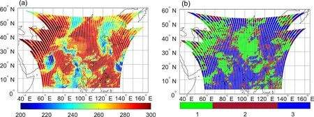
Fig. 2. The GIIRS-observed brightness temperatures (units: K) of channel 320 (900 cm-1) (a) and the cloud detection results (b) in the China area on 10 August 2019, from 1200 to 1340 UTC.
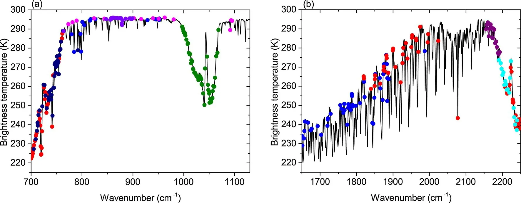
Fig. 3. Selected retrieval channels at the GIIRS’s LWIR band (a) and the MWIR band (b).
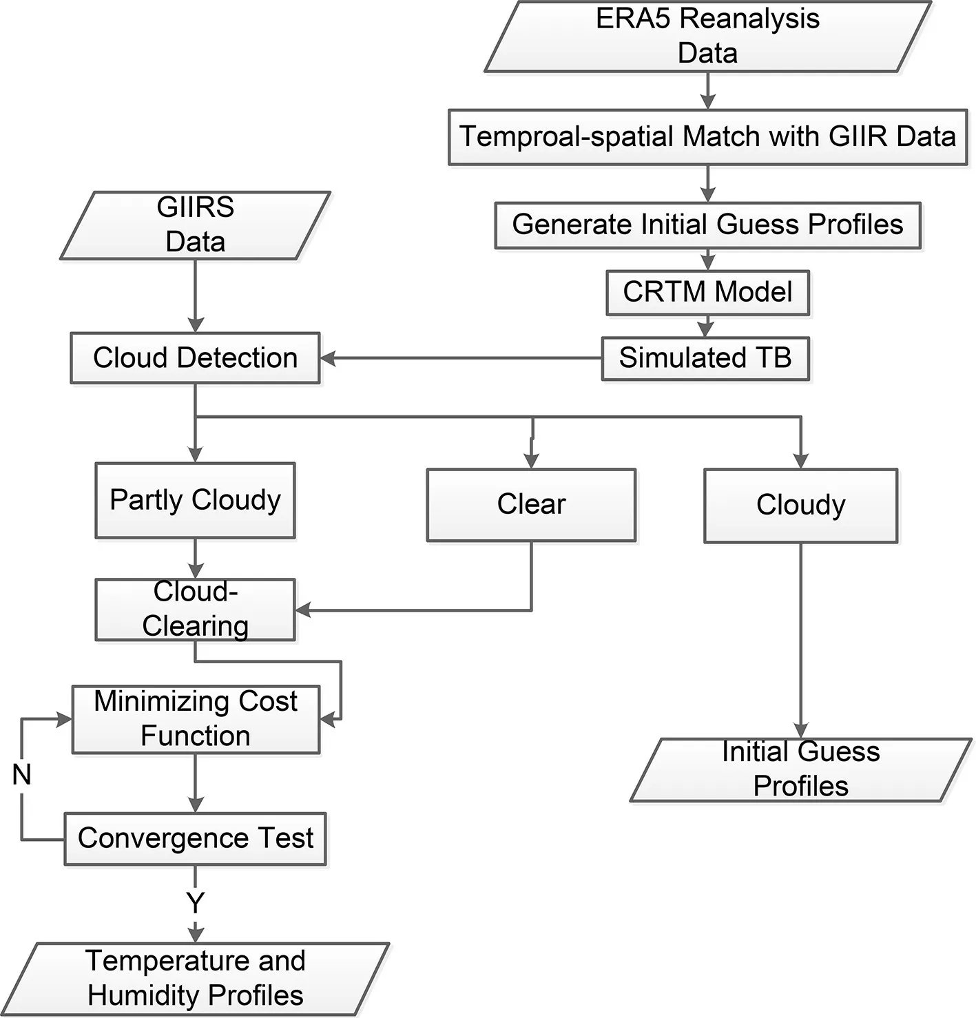
Fig. 4. Flow chart of the 1D-Var retrieval process for the GIIRS.
4. Results and discussion
The radiosonde data available at the CMDC were used as a reference to validate the quality of the atmospheric profiles retrieved in this study and the FY-4A operational L2 temperature profiles were obtained from the NSMC. To obtain a sufficient sample size to evaluate the retrieval accuracy,four months of radiosonde data in December 2019 and January, July, and August 2020 were selected for validation. The coordinates of each GIIRS FOV are matched with those of each upper air sounding station. Sample pairs that meet the following distance threshold criterion are obtained by setting a threshold of distance on the surface of a sphere (Yu et al., 2020):

where l atG, l onGand l atS, l onSrepresent the longitude and latitude of the GIIRS FOV and the sounding station, respectively and R represents the radius of the Earth (6371 km). A distance threshold of 16 km is set according to the spatial resolution of the GIIRS. In addition to spatial matching, the observation times should be taken into consideration. The radiosonde data are received, twice daily, at 0000 and 1200 UTC. The retrievals are performed half an hour before and after these times. After spatial and temporal matching, 81 pair stations in China were selected, and the total number of samples for each month was 4860. The parameter describing humidity in the radiosonde data is the dew point temperature. To facilitate the comparison of the humidity retrieval results, the temperature of the dew point is converted to the specific humidity, q, following the equations:

where e represents vapor pressure; Tdrepresents the dew point temperature, and p is the pressure.
The statistical metrics used to evaluate the accuracy of the inversion profiles include the mean bias (MB) and root mean square error (RMSE), which are defined as follows:

where n represents the number of samples; xiis the radiosonde value, and xi′is the retrieval value.
4.1. Impact of channel selection
To compare the retrieval accuracy and computational efficiency using the selected 329 channels described in section 3.4 with an approach that uses all 1650 GIIRS channels, we take every five days in July 2020 as an example. There are 149 radiosonde data points under clear conditions and 742 radiosonde data points under partly cloudy conditions. The retrieved results using the 329 channels plus all remaining longwave channels within 700-774.375 cm-1(370 channels) were also analyzed statistically. The MB and RMSE profiles for temperature obtained using 329, 370, and 1650 channels are shown in Fig. 5. In terms of RMSE, the retrievals based on 329 channels have better accuracy compared to those using 370 and 1650 channels from surface to 70 hPa under both clear and partly cloudy conditions, while the MB of all 1650 channels is less than optimal. This is likely due to the high channel correlation and information redundancy of the hyperspectral infrared sounding channels. In the stratosphere, the RMSE and MB of all sets are higher, which may be attributed to a greater tendency for the radiosonde balloon to float with increasing height. Another reason is that there are few channels whose peak height of WF is located between 50-200 hPa regardless of whether 1650 channels or the selected channels are used. Above 70 hPa, the use of 1650 channels shows a better performance. This is because ozone channels (1000 -1100 cm-1) whose WF peak altitudes are located near 30 hPa could provide more temperature information in the upper levels; fewer ozone channels are selected in the 329 and 370 channel sets.
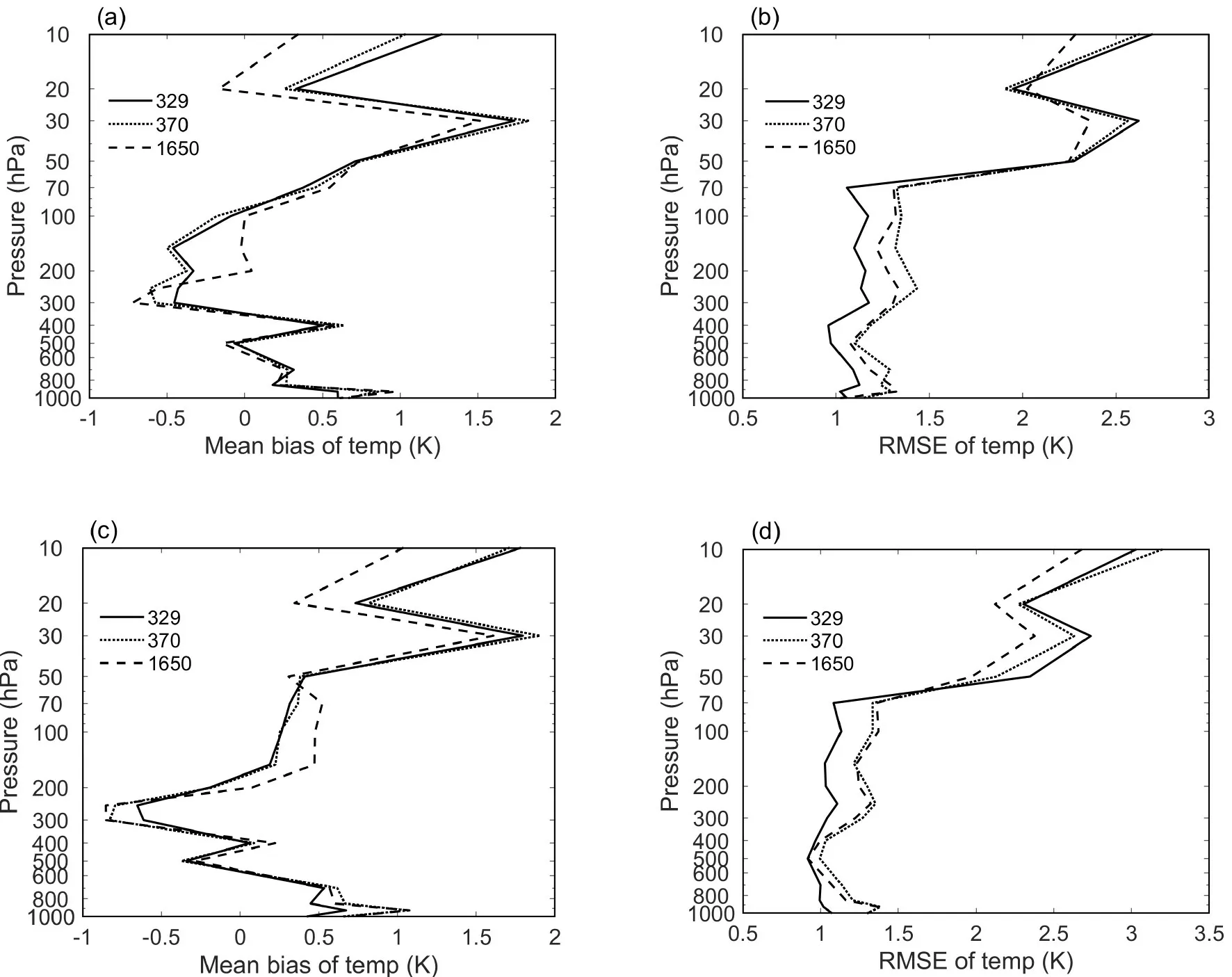
Fig. 5. The MB (a) and RMSE (b) profiles of the retrieved temperature under clear conditions and the MB (c) and RMSE (d) profiles under partly cloudy conditions in July 2020.
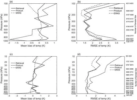
Fig. 6. The MB (a) and RMSE (b) profiles of the inversion temperatures under clear conditions in December 2019 and January 2020 and the MB (c) and RMSE (d) profiles of the inversion temperatures under clear conditions in July and August 2020. The solid lines represent the results retrieved from the 1D-Var approach, the dashed lines represent the ERA5 reanalysis data, and the dash-dot lines represent the NSMC L2 operational products.
The average retrieval time of one FOV is 5.05 seconds using the selected 329 channels and 5.97 seconds for the full channel set. The run time for the entire China area is about 2.5 hours for selected channels, saving about 15%time compared to the 1650 channels.
4.2. Under clear skies
Taking radiosonde data as true values, the MB and RMSE profiles of the temperatures retrieved by the 1D-Var approach, described in this paper, and the L2 operational products from the NSMC and the ERA5 reanalysis data,used as initial guess field under clear conditions in December 2019 and January 2020 (winter season), are given in Figs. 6a and 6b respectively. Figures 6c and 6d show the MB and RMSE profiles for July and August 2020 (summer season). The solid lines represent the results retrieved from the 1D-Var approach, the dashed lines represent the ERA5 reanalysis data, and the dash-dot lines represent the NSMC L2 operational products. Due to the lack of radiosonde data above 100 hPa in the winter season, the results are shown only from 1000 hPa to 100 hPa in Figs. 6a and 6b), while the errors from 1000 hPa to 10 hPa are presented in Figs. 6c and 6d. The number of sample sizes used to calculate the MBs and RMSEs at each pressure level is given on the right vertical coordinate. The number in the first column represents both the retrieved results and the ERA5 data, and the number in the second column represents the L2 operational products. The number of sample sizes at each level decreases as the altitude decreases because radiosonde data near the surface are not as plentiful compared to those at high levels. It can clearly be seen that there are large negative deviations, up to 2 K, for the NSMC L2 operational products below 800 hPa in both winter and summer. The most accurate temperature retrievals for the 1D-Var approach and L2 operational products are both between 800 hPa and 200 hPa, with MBs between ±0.5 K. The MBs of the results retrieved from the 1D-Var approach are less than those of the L2 operational products above 200 hPa. The RMSEs of the 1D-Var-retrieved temperatures are less than those of the L2 operational products for the whole atmosphere, especially in summer. The RMSEs of the temperatures retrieved from the 1D-Var approach are approximately 1 K in summer, except near the ground. In the winter season, the RMSEs of the 1D-Var-retrieved temperatures are slightly higher, from 1.5 K to 2 K. Compared with the ERA5 reanalysis data, the retrieved results are improved between 800 hPa and 300 hPa for both the winter and summer seasons. The RMSEs of the temperatures retrieved from the 1D-Var approach decrease about 0.1 K compared with the ERA5 data from 800 hPa to 300 hPa, but the MBs of the retrievals are larger in the whole atmosphere. Above 200 hPa, the RMSEs of the retrieved temperatures increase by more than 2 K. These are similar to the errors that appear in the L2 products. This may have resulted due to the following three reasons: there are few temperature sounding channels whose WF peak values are located near or above the upper troposphere, errors are caused by sounding balloons floating at high altitudes, and the number of samples above the upper troposphere is reduced with limited radiosonde data. Figure 7 shows scatter plots of the temperatures received with the radiosondes. Figures 7a and 7c indicate that the correlation coefficient between the 1D-Var retrievals and the radiosonde data is 0.992 in winter and 0.993 in summer, which indicates a high correlation. The average RMSE of the whole troposphere in winter is 2.045 K, and the MB is 0.126 K, while in summer, the average RMSE of the whole atmosphere is 1.388 K and the MB is 0.23 K. The retrieved values and radiosonde values are evenly distributed on both sides of the line y=x. The scatter plots of the NSMC L2 products in Figs. 7b and 7d show slightly higher RMSEs, with 2.243 K in winter and 2.302 K in summer.
Because humidity profiles are not provided in the L2 operational products from the NSMC, only the performance of the retrieved humidity profiles and ERA5 reanalysis data was evaluated through comparison to the radiosonde data. The distributions of the RMSE and MB profiles of the retrieved humidity in the troposphere are shown in Fig. 8. The solid line in Fig. 8 represents the RMSE, while the dashed line represents the MB. As shown in Fig. 8, the highest RMSE (approximately 2.5 g kg-1) occurs near the surface at 925 hPa in both winter and summer. Except for the near-surface level, the RMSE of each level in the troposphere is less than 2 g kg-1and decreases with height. Meanwhile, the dash-dot line and the dotted line stand for the RMSE and MB of the ERA5 humidity in Fig. 8, respectively. The retrieved humidity appears to be in better agreement with the radiosonde data than the ERA5 data between 800 hPa and 300 hPa in both the winter and summer seasons. Scatterplots of the retrieved humidity data and the radiosonde data are given in Fig. 9. The results show that the correlation coefficient is 0.926 in winter and 0.948 in summer.The retrieved values and radiosonde values show a good correlation. In winter, the mean RMSE of the humidity in the troposphere is 0.748 g kg-1, and the MB is -0.027 g kg-1; in summer, the mean RMSE is 1.040 g kg-1, and the MB is 0.217 g kg-1. The retrieval accuracy of humidity in winter is slightly better than that in summer. Noteworthy is the persistent underestimation of humidity in summer in Fig. 9b,which is consistent with the fact that water vapor content that is excessively high or low in the atmosphere is not conducive to improving retrieval accuracy (Zong, 2020).

Fig. 7. Scatterplots of retrieved (a) and level-2 product (b) temperatures with radiosonde observations for the whole atmosphere under clear-sky conditions in December 2019 and January 2020, and the same plots for retrieved (c) and level-2 product (d) temperatures in July and August 2020.
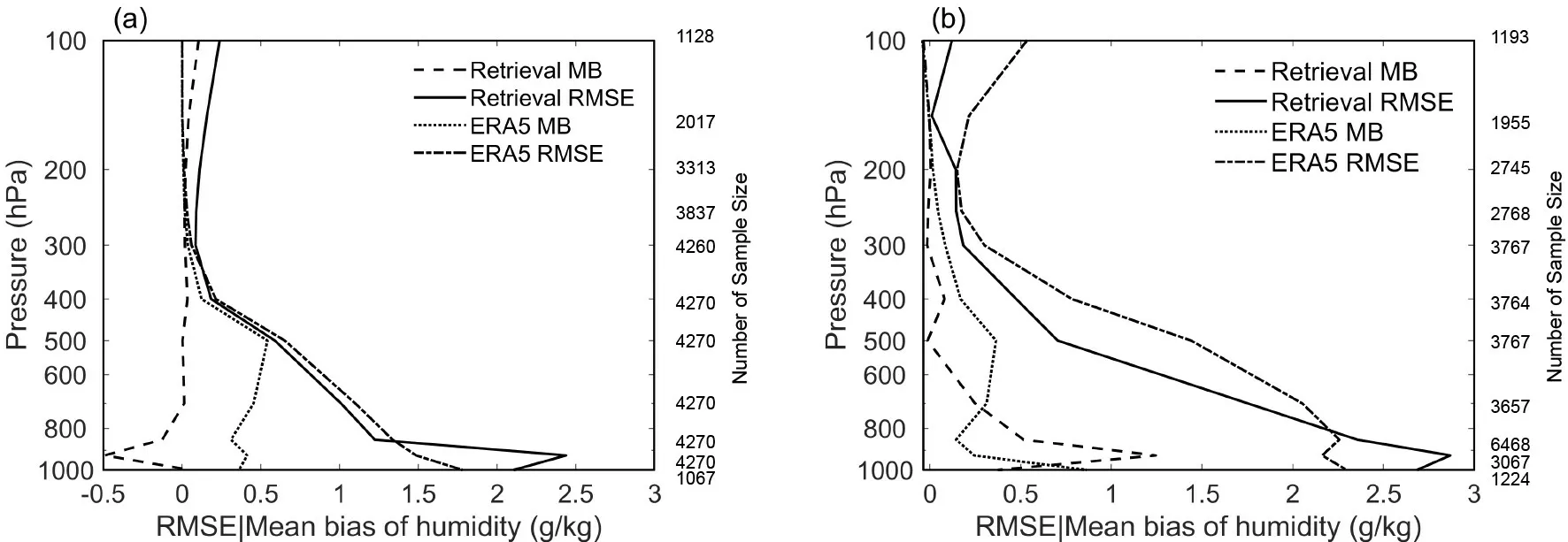
Fig. 8. Errors of the humidity profiles under clear conditions in December 2019 and January 2020 (a) and in July and August 2020(b).
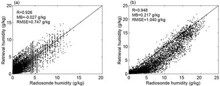
Fig. 9. Scatterplots of the humidity profiles in the troposphere under clear conditions in December 2019 and January 2020 (a) and in July and August 2020 (b).
4.3. Under partly cloudy conditions
Among the relevant characteristics of the NSMC L2 operational products are the missing temperature values at altitudes below the cloud top and the lacking humidity profiles when the FOV is assigned as cloudy according to the L2 cloud mask products. An example of a single-profile temperature and humidity retrieval from the L2 operational products compared with a radiosonde profile (station number 54511)under partly cloudy conditions on 1 August 2020 at 0000 UTC is presented in Figs. 10a and 10b, respectively. The dashed line in Fig. 10 represents the profile retrieved by the 1D-Var approach, the dotted dashed line represents the L2 operational product, and the solid line represents the radiosonde observations. The L2 temperature profile below 300 hPa has no value, and the 1D-Var-retrieved temperature profile is closer to the radiosonde profile than it is to the L2 profile in both the troposphere and stratosphere (Fig. 10a). The humidity comparison is illustrated in Fig. 10b. The retrieved humidity profile is still very close to the radiosonde profile.Fig. 10c displays the performance of the minimization of the cost function for this single-profile retrieval. The χ2values versus iteration number for this single-profile were recorded. The red line represents the iteration criteria 0.7. It can be seen that its value decreases along with the increase of iterations; the criterion is met after the seventh iteration.
Figures 11a and 11b show the MBs and RMSEs, respectively, of the 1D-Var-retrieved temperature profiles, the ERA reanalysis data, and the L2 products from the NSMC compared with radiosonde data under partly cloudy conditions in December 2019 and January 2020 (winter season).Figures 11c and 11d show the MBs and RMSEs, respectively, in July and August 2020 (summer season). The number of samples at each pressure level is given on the right side of Figs. 11b and 11. The first column number represents both the retrieved results and the ERA5 data, and the second column number represents the sample size of the L2 operational products. The sample size of the L2 operational products decreases sharply with decreasing height because of the limited data below the cloud top, especially in Fig. 11d.The L2 temperature profile is available only at altitudes above the cloud top under partly cloudy conditions. In contrast, the 1D-Var-retrieved temperatures can be produced through the entire atmosphere under partly cloudy conditions. Whether in winter or summer, the RMSEs of the temperature profiles retrieved from 1D-Var, at all vertical levels, are far less than those of the L2 products. Compared with Figs. 6 and 11, it is evident that the temperature retrieval accuracy under partly cloudy conditions is similar to that under clear conditions. The most accurate retrievals occur between 800 hPa and 300 hPa, and the RMSE value was reported to be approximately 1 K. A comparison between the retrievals and the radiosonde data shows smaller RMSE values between 800 hPa and 300 hPa than does the comparison between the ERA5 reanalysis data and radiosonde data. Above 200 hPa, the higher the altitude, the larger the deviation between the retrievals and ERA5. The inversion accuracy in winter is slightly worse than that in summer.
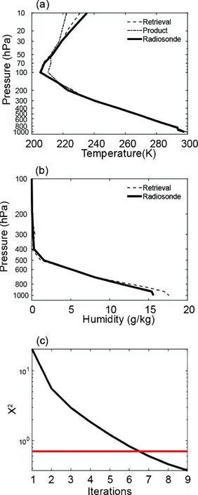
Fig. 10. An example of temperature (a) and humidity (b)retrievals compared with radiosonde data under partly cloudy conditions and χ2 values versus iteration number (c) on 1 August 2020 at 0000 UTC.
Scatterplots of the retrieved temperature and L2 products under partly cloudy conditions are shown in Fig. 12.The statistical correlation coefficient, MB, and RMSE of the 1D-Var method are all smaller than those of the L2 product.This again shows that the 1D-Var inversion accuracy is higher than that of the operational method. The correlation coefficient between the retrievals and the radiosonde data is 0.966 in winter and 0.991 in summer. In winter, the average temperature RMSE is 2.371 K, and the MB is 0.384 K;in summer, the average RMSE is 1.404 K and the MB is 0.310 K. Under partly cloudy conditions, the retrieved temperatures are generally higher than the target temperatures, similar to the results obtained under clear-sky conditions.
Figure 13 shows the RMSE and MB profiles of the humidity profile obtained from 1D-Var and ERA5 reanalysis data under partly cloudy conditions in the troposphere.No humidity profiles were obtained from the NSMC products. The solid line represents the RMSE, while the dashed line represents the MB of retrieved humidity. The dash-dot line and the dotted line stand for the RMSE and MB of the ERA5 humidity, respectively. As shown in Fig. 13,the highest RMSE (approximately 3 g kg-1) occurs near the surface in both winter and summer, and the deviation tends to decrease with increasing height. The RMSEs of the retrieved humidity are also smaller than the ERA5 humidity between 800 hPa and 300 hPa. Scatterplots of the retrieved humidity with the radiosonde data are given in Fig. 14. The correlation coefficient is 0.892 in winter and 0.953 in summer. The mean winter RMSE of the humidity profile is 0.917 g kg-1, and the RMSE value is 1.567 g kg-1in summer.

Fig. 11. The MB (a) and RMSE (b) profiles of the inversion temperatures under partly cloudy conditions in December 2019 and January 2020 and the MB (c) and RMSE (d) profiles of the inversion temperatures under partly cloudy conditions in July and August 2020. The solid lines represent the results retrieved from the 1D-Var approach,the dashed lines represent the ERA5 reanalysis data, and the dash-dot lines represent the NSMC Level-2 operational products.
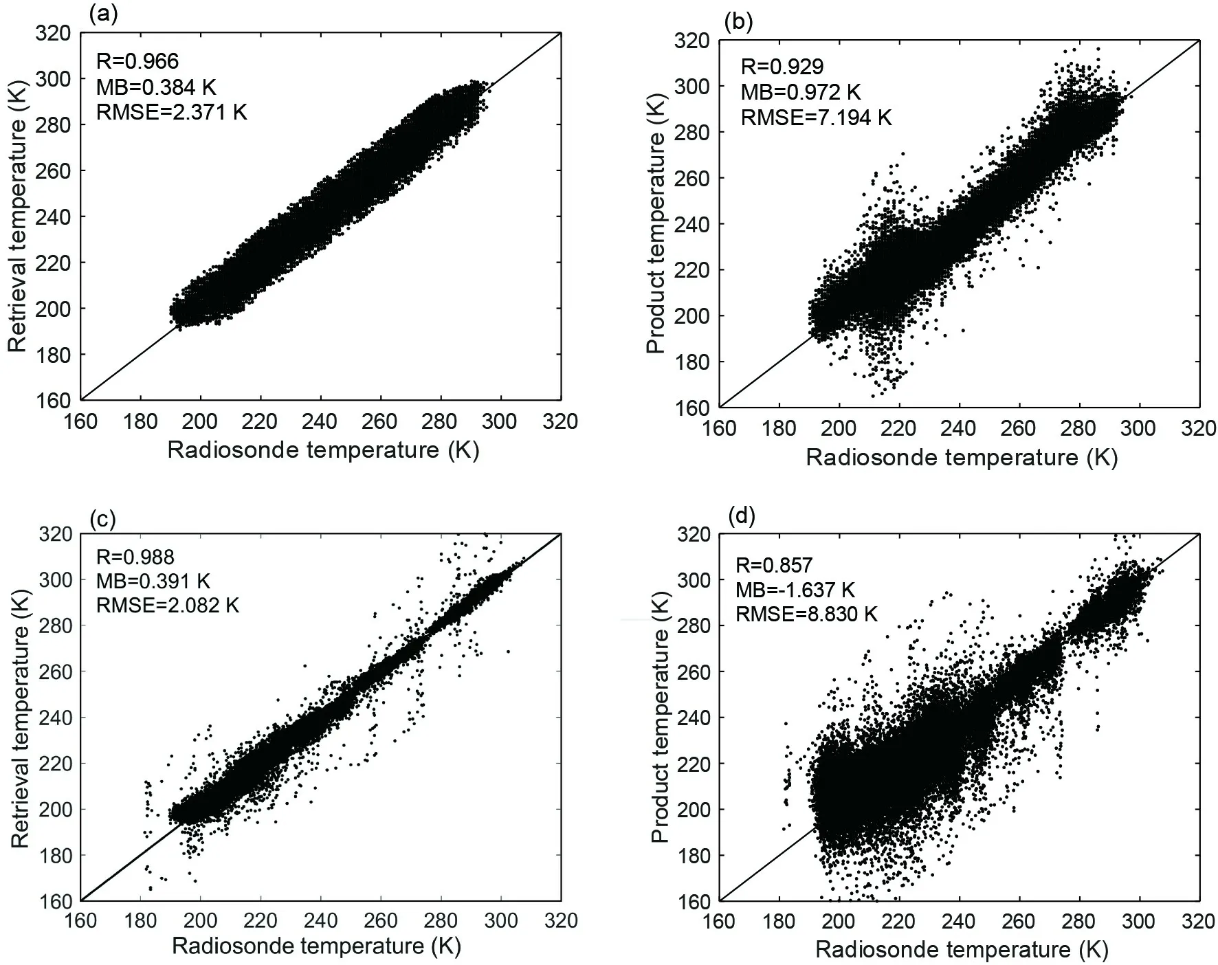
Fig. 12. Scatterplots of retrieved (a) and level-2 product (b) temperatures with radiosonde observations for the whole atmosphere under partly cloudy conditions in December 2019 and January 2020 and the same plots of retrieved (c) and level-2 product (d) temperatures in July and August 2020.

Fig. 13. The humidity error profiles under partly cloudy conditions in December 2019 and January 2020 (a) and in July and August 2020 (b).

Fig. 14. Scatterplots of the humidity profiles in the troposphere under partly cloudy conditions in December 2019 and January 2020 (a) and in July and August 2020 (b).
The possible error sources in the retrieval process are accounted for upon investigating the retrieval uncertainties which may include, but are not limited to: too few temperature sounding channels whose WF peak values are located near the upper-troposphere (as mentioned in section 4.1)account for the inaccuracy in the high levels; the cloud detection is not accurate causing the clear-sky FOVs and partlycloudy FOVs not to be completely detected; in temporal matching, the inputs for the forward model adopted the initial profiles at 0000 and 1200 UTC and the corresponding GIIRS data had deviations of up to one hour; in spatial matching, the satellite FOVs and the spatial grid point of the ERA5 reanalysis data are not completely spatially matched.
5. Conclusions
As the first infrared hyperspectral sounder onboard a geostationary weather satellite, FY-4A’s GIIRS can provide three-dimensional atmospheric temperature and humidity fields with high scanning frequencies and spatial resolutions. Therefore, the improvement of retrieval precisions based on hyperspectral infrared data, especially on stationary satellite platforms, is of great significance. The 1D-Var physical retrieval algorithm is used in this paper to simultaneously retrieve the temperature and humidity profiles under both clear-sky and partly cloudy conditions. Collocated radiosonde observations from upper-air stations in the China area are used to validate the data quality of the retrieved temperature and humidity profiles along with the NSMC Level-2(L2) operational products during the periods from December 2019 to January 2020 and from July 2020 to August 2020. The results are as follows:
(1) The RMSE accuracy of the 1D-Var temperature retrievals is within 2 K for the entire depth of the troposphere except for near the surface under clear-sky conditions. The most accurate temperature retrievals are between 800 hPa and 200 hPa with RMSEs less than 1 K. The correlation coefficients between the 1D-Var retrievals and radiosonde data are all approximately 0.99, and the retrieved temperature profile is closer to the radiosonde data than are the L2 products in both winter and summer.
(2) The temperature values in the NSMC L2 operational products are missing at altitudes below the cloud top;temperature and humidity profiles can be produced at each vertical level by the 1D-Var method under partly cloudy skies.
(3) The retrieval accuracy under partly cloudy conditions can maintain the same performance as that under clear conditions. The temperature RMSE profiles at all vertical levels from 1D-Var are far less than those of the L2 products. The mean RMSE in the troposphere is within 2 K.
(4) Only the performance of the retrieved humidity profiles was evaluated in comparison to the radiosonde data since humidity profiles are not provided in the NSMC L2 operational products. The average RMSE of the retrieved humidity profiles is within 2 g kg-1, whether under clear or partly cloudy skies.
(5) The temperature and humidity retrievals show an improved performance compared to the ERA5 reanalysis data between 800 hPa and 300 hPa both in winter and summer seasons, whether under clear or cloudy sky conditions.Furthermore, the retrievals can provide the atmospheric profiles with a higher temporal resolution than the ERA5 reanalysis data.
Overall, temperature and humidity profiles can be provided by the 1D-Var physical retrieval algorithm with high precision under all weather conditions based on the output of the hyperspectral infrared imager uploaded on the geostationary satellite platform.
Acknowledgements.The authors would like to thank the editor and reviewers for their helpful comments on the manuscript.This work was supported in part by the National Key Research and Development Program of China under Grant No.2018YFC1507302, in part by the National Natural Science Foundation of China under Grant No. 41975028.
 Advances in Atmospheric Sciences2022年3期
- Advances in Atmospheric Sciences的其它文章
- Electronic Supplementary Material to:A New Index Developed for Fast Diagnosis of Meteorological Roles in Ground-Level Ozone Variations*
- Electronic Supplementary Material to:Seasonal Prediction of Summer Precipitation over East Africa Using NUIST-CFS1.0*
- Electronic Supplementary Material to:Detection and Attribution of Changes in Thermal Discomfort over China during 1961-2014 and Future Projections*
- The 16th Workshop on Antarctic Meteorology and Climate and 6th Year of Polar Prediction in the Southern Hemisphere Meeting
- A New Method of Significance Testing for Correlation-Coefficient Fields and Its Application
- Observations of Dynamic Turbulence in the Lower Stratosphere over Inner Mongolia Using a High-resolution Balloon Sensor Constant Temperature Anemometer
