A New Method of Significance Testing for Correlation-Coefficient Fields and Its Application
Xiaojuan SUN, Siyan LI, Julian X. L WANG, Panxing WANG, and Dong GUO
1Key Laboratory of Meteorological Disaster, Ministry of Education/ Collaborative Innovation Center on Forecast and Evaluation of Meteorological Disasters, Nanjing University of Information Science and Technology, Nanjing 210044, China
2Nanjing Xindan Institute of Meteorological Science and Technology, Nanjing 210044, China
3Air Resources Laboratory, National Oceanic and Atmospheric Administration, Silver Spring, Maryland, 20901, USA
ABSTRACT Correlation-coefficient fields are widely used in short-term climate prediction research. The most frequently used significance test method for the correlation-coefficient field was proposed by Livezey, in which the number of significantcorrelation lattice (station) points on the correlation coherence map is used as the statistic. However, the method is based on two assumptions: (1) the spatial distribution of the lattice (station) points is uniform; and (2) there is no correlation between the physical quantities in the correlation-coefficient field. However, in reality, the above two assumptions are not valid.Therefore, we designed a more reasonable method for significance testing of the correlation-coefficient field. Specifically, a new statistic, the significant-correlation area, is introduced to eliminate the inhomogeneity of the grid (station)-point distribution, and an empirical Monte Carlo method is employed to eliminate the spatial correlation of the matrix.Subsequently, the new significance test was used for simultaneous correlation-coefficient fields between intensities of the atmospheric activity center in the Northern Hemisphere and temperature/precipitation in China. The results show that the new method is more reasonable than the Livezey method.
Key words: correlation-coefficient field, significant-correlation area, empirical Monte Carlo method, significance test
1. Introduction
Considering a geographical region D covered by a lattice (site) network composed of m grid lattices (sites)( s=1,...,m), the field r composed of the correlation coefficient rs,s=1,...,m in the lattice (site) network becomes the distribution field of the correlation coefficient (still noted as r). r can be the distribution field of the correlation coefficient between the time series of a factor or factors xq,q=1,...,n (noted as x) and the time series of the previous factor field yq,q=1,...,n (noted as Ym×n) in D, which can also be the local correlation-coefficient distribution field of time series Xm×nand Ym×nof the two factor fields on D. In the analysis of atmospheric circulation and climate anomalies, r is widely used for analyzing the correlation between atmospheric circulation and contemporaneous or lagged climatic anomalies (Feng, 1978; Chen and Song,2000; Gong et al., 2002; Hua and Ma, 2009; Ma et al.,2009; Wu et al., 2011; Huang and Wang, 2012; Xu and Wu,2012; Liu et al., 2015).
In order to infer whether there is a correlation between the parent population from r of sample x(X)~Y, r needs to be tested for significance. Livezey and Chen (1983)developed an r significance test method (known as the Livezey method), which assumes that k of m correlation coefficients rs,s=1,...,m constituting r pass the significance test of reliability α, and k is the number of significant-correlation lattices (stations). Assuming that the matrix of x(X) and Y are not correlated, the critical value kαof k can be determined by m and α according to Bernoulli’s theorem. When k≥kα, the correlation-coefficient distribution field passes the significance test of reliability α.
However, the Livezey method implies that kαis based on two assumptions: (1) a uniform space of lattice (site)points; and (2) the matrix space of the local sequence X and Y has no correlation. However, for all planetary-scale twodimensional lattice (site) networks, neither of these assumptions is true. Therefore, the Livezey method for r significance testing has defects.
This paper is based on research results regarding the correction of spatial homogenization of climatic data (Chung and Nigam, 1999; Luo et al., 2011) and introduces a new statistic, the significant-correlation area of r, which is used to replace the number of total stations k of the significant correlation of r in the Livezey method and eliminate the influence of the lattice (site) network being uneven in reality. Furthermore, the Monte Carlo method to test the significance ofis replaced with an empirical Monte Carlo method, eliminating the influence of the X(Y) parent space correlation, so as to obtain a reasonable and operable new method of r significance testing.
2. Methods
2.1. Definition and calculation of significant-correlation area
2.1.1. The definition of
The correlation-coefficient field r is given in the field area Ω, the signi(fic)a nt-correlation in t(he) regionis (|r|≥rα), andis the area ofis the significant-correlation region of r, andis the significant-correlation area of r.
2.1.2. The calculation of
Fields of r used in atmospheric circulation or climate analysis are obtained from the discretized data given on the lattice (site) network, and the most commonly used lattice network is a rectangular network with uniform spacing on plane λ-φ (λ is the longitude, φ is the latitude). Figure 1a is a uniform grid distance rectangular lattice network in the Northern Hemisphere, and the network area is D =2πa2(a is the radius). Figure 1b shows a 160-station network in China with an area of about 9.6 million km2. Obviously, the distribution of lattice points on the network is uneven. In order to calculate, it is first necessary to give the measurement method of the lattice network inhomogeneity. Luo et al.(2011) introduced the element area dsof the s-th lattice(site), which is the part of the domain area D represented by the s-th lattice (site). The larger (smaller) dsis, the sparser(denser) the dot distribution is near point s. dsis the basis for calculating the area of the significant-correlation area,and its algorithm should be given first.
(1) Calculation of element area ds
Chung and Nigam (1999) pointed out that the element area of the lattice point located at latitude φ on the lattice network in Fig. 1a was proportional to cosφ. Figure 1a shows the uniform spacing on the λ -φ plane of the Northern Hemisphere (Δ λandΔφ are constant). The zonal lattice number is u(Δλ=2π/u), and the meridional lattice number is(v+1)(Δφ=π/2v). The two-dimensional lattice point ordinal number (i,j)=(0,0) is taken on the intersection point (λ,φ)=(0,0) between the prime meridian and the equator, and by using Fig. 2, the corresponding element area can be easily written (i is the longitude coordinates, j is the latitude coordinates):

Fig. 1. Example of lattice (site) network. (a) Uniform grid distance rectangular lattice network in the Northern Hemisphere(Δ λ,Δφ=π/18);(b) 160-station network in China (Wang et al., 2011).
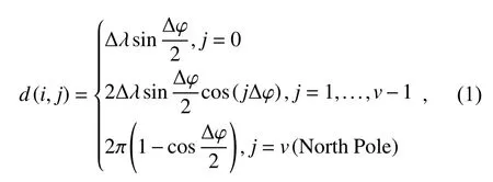
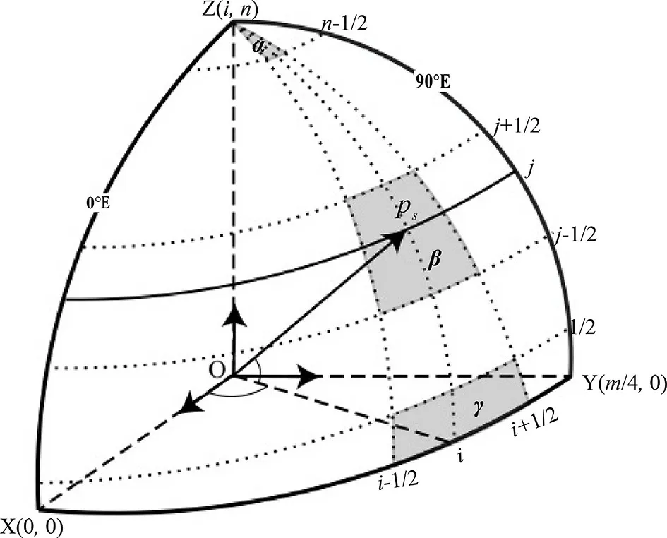
Fig. 2. A schematic diagram of the calculation of the area of s lattice element. The shaded area of the Arctic is only d s/4.
where the units of Δ λ and Δ φ are radians (rad), and the units of d(i,j) and d(i,j) are the radius of the Earth squared.Because Δλ is constant, d(i,j) only changes with j. Using the relation S~(i, j),

where d(i,j) can be easily converted to ds. Note that the North Pole is processed into u lattice points, ds=m=u(v+1), Δλ=Δφ=π/1 8, u= 36, v=9, and m=u(v+1)=360.
Luo et al. (2011) presented the calculation scheme of S station area dson a Chinese 160-station network (Fig. 1b),which is briefly introduced here with the help of Fig. 3. In the figure, S represents the test station located at (λs,φs).The shaded area in Fig. 3 is the spherical part of the spherical crown with S as the pole, and the area S0is called the area of the crown [(S0=2π(1-cosθ)a2, where a is the radius of the Earth and θ =∠SOS*is the center angle corresponding to the pole of the spherical cap to the edge point)].For the selected S0, S station crown area Ωsis determined,and its area is S0. The number of stations in the statistics is determined to be, and then the area Dsthat belongs to the coverage area of station network Ωsis calculated. Thus,the area dsof station element S and the density of the station network are obtained, which are defined as:
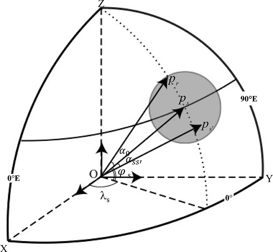
Fig. 3. A schematic diagram of the calculation of the area of s station. The shaded area is Ω s.

Figure 4 is the diagram representing the calculation of dsand msfor the Lanzhou (inland), Altay (land border), and Shanghai (ocean boundary) stations. For the inland station,Ds= 1, and for the boundary station, Ds< 1. Table 1 shows ds,ms, and the intermediate calculation results ofand Dsfor the three stations.
Table 1. The , D s, ds , and m s of the Lanzhou, Altay, and Shanghai stations.

Table 1. The , D s, ds , and m s of the Lanzhou, Altay, and Shanghai stations.
(2) Calculate of the significant-correlation area D
Figure 1 shows the correlation-coefficient field r in the lattice (site) network composed of m phase relationship values rs. The significance test of reliability α is carried out for each rs, where k-th rsare significant. We introduce 0 and 1 functions,

in which we take 1 through the test lattice (site) point ps; otherwise, we take 0. Thus, the formula for calculating the area of the significant-correlation area in the correlation-coefficient field is obtained as

2.2. Significance test of correlation-coefficient field r by the empirical Monte Carlo method
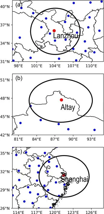
Fi g. 4. A schematic diagram of the structure of three types of stations. The elliptical line is the Ωs boundary, the shallow shadow area is the ocean, the deep shadow area is the land, and the white curve is the land boundary/sea land demarcation line.(a) Lanzhou (inland) station, (b) Aletai (land border) station,and (c) Shanghai (ocean boundary) station.
2.2.1. EMC method
r is the correlation-coefficient distribution fields of the time series x and field series Y or the local correlation-coefficient distribution fields of the sequence of fields X and Y in the same grid (site) network at the same time (or delayed) in time series q =1,...,n. x, X, and Y are expressed as

wherexqis the t-th time value of sequence x, andxqandyqare thet-th time fields of field orders X and Y. The test steps of reliability α of r using the EMC method are as follows:
(1) According to the method described in section 2, the significant-correlation areaof sample correlation-coefficient field r is found.
(2) The sample sequencexq,q=1,...,norxq,q=1,...,nis randomly selected L times by a random function, where L = 1000 or more. Then, the correlation-coefficient field ofxl(orXl),l=1,...,L, and Y are found, and the following is obtained:

(4) The significance of r is tested with statistic: Ifthen r is significant with respect to α under the reliability, and x(X) and Y are from the relevant parent; otherwise, r is not significant, and x(X) and Y come from an uncorrelated parent.
The key of the EMC method is to use the random sequence of the sample sequence x(X) to generate its simulated sequencexl(Xl), which is the basis of the word “empirical” in its name. This process makes the statistical properties ofxl(Xl) closest to the sample and the statistical properties of the sample closest to its parent. For example, therlobtained by the EMC method in step (2) should be well organized. Therefore, the EMC significance test of r considers the spatial correlation of X (or Y).
So that evening, when the Princess came once more with her sleeping-drink, he pretended to drink, but threw it away behind him, for he suspected that it was a sleeping-drink
2.2.2. Livezey method
For the 160-station network of China, when the reliability α=0.05 and L=1000, the critical value of k for the number of significantly correlated stations of in the correlogram isk0.05= 13 (Wang et al., 2007). Whenk>k0.05, r passes the significance test, and x(X) and Y come from the correlation matrix.
3. Practical examples of application
According to the method of Sun et al. (2015), we obtained the intensity sequencePt,t=1,...,70 (P) of five atmospheric activity centers (ACAs) during a 70-yr period(1951-2020) in the Northern Hemisphere in winter, which is x in Eq. (5). Then, the temperature and precipitation field sequences (T and R) were obtained at 160 stations in Chinaduring the same period, which is Y in Eq. (5). Figures 5 and 6 show the simultaneous correlation-coefficient field r of x-T and x-R, respectively.
Table 2 shows the significance test results of the EMC method with the areaand α = 0.05 of the significance test area in Figs. 4 and 5. Two qualitative ACAs in the North Atlantic (Iceland low and North Atlantic High) and the Mongolia High intensity in eastern Eurasia are significantly correlated with the corresponding winter temperature in China.Quantitatively, the correlation between the Mongolian High and temperature is the strongest, followed by the Icelandic Low and the North Atlantic High. The correlation between intensity and China’s winter precipitation in the same period is much weaker, and only the Icelandic Low intensity is significantly correlated with China’s precipitation in the same period. The above conclusions are consistent with the size of the significant-correlation area in Figs. 5 and 6.
Table 3 shows the Livezey significance test results of the number of significantly correlated stations k and α=0.05 in Figs. 5 and 6. It can be seen that the test results of P-T are consistent. However, the test results of P-R vary greatly.Regarding P-R, in addition to the Icelandic Low, the Mongolian High, Aleutian Low, and North Pacific High were also significantly correlated. As can be seen from Figs. 6c-e,although the area of the significant-correlation area above them is small, they are all located in the dense area of the site in Fig. 1b. The inhomogeneity of the station network seriously affects the significance test of r.
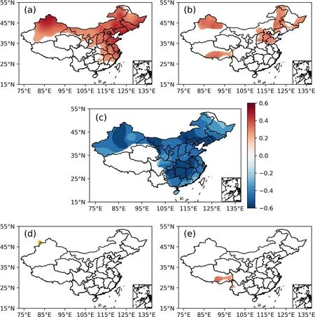
Fig. 5. Correlations between ACA intensity index in the Northern Hemisphere and temperature at 160 stations in China in winter from 1951 to 2020. The shaded area is the significant-correlation area that passes the t test at the α=0.05 level. (a) Iceland low. (b) North Atlantic High. (c) Mongolia High. (d) Aleutian Low. (e) North Pacific High.
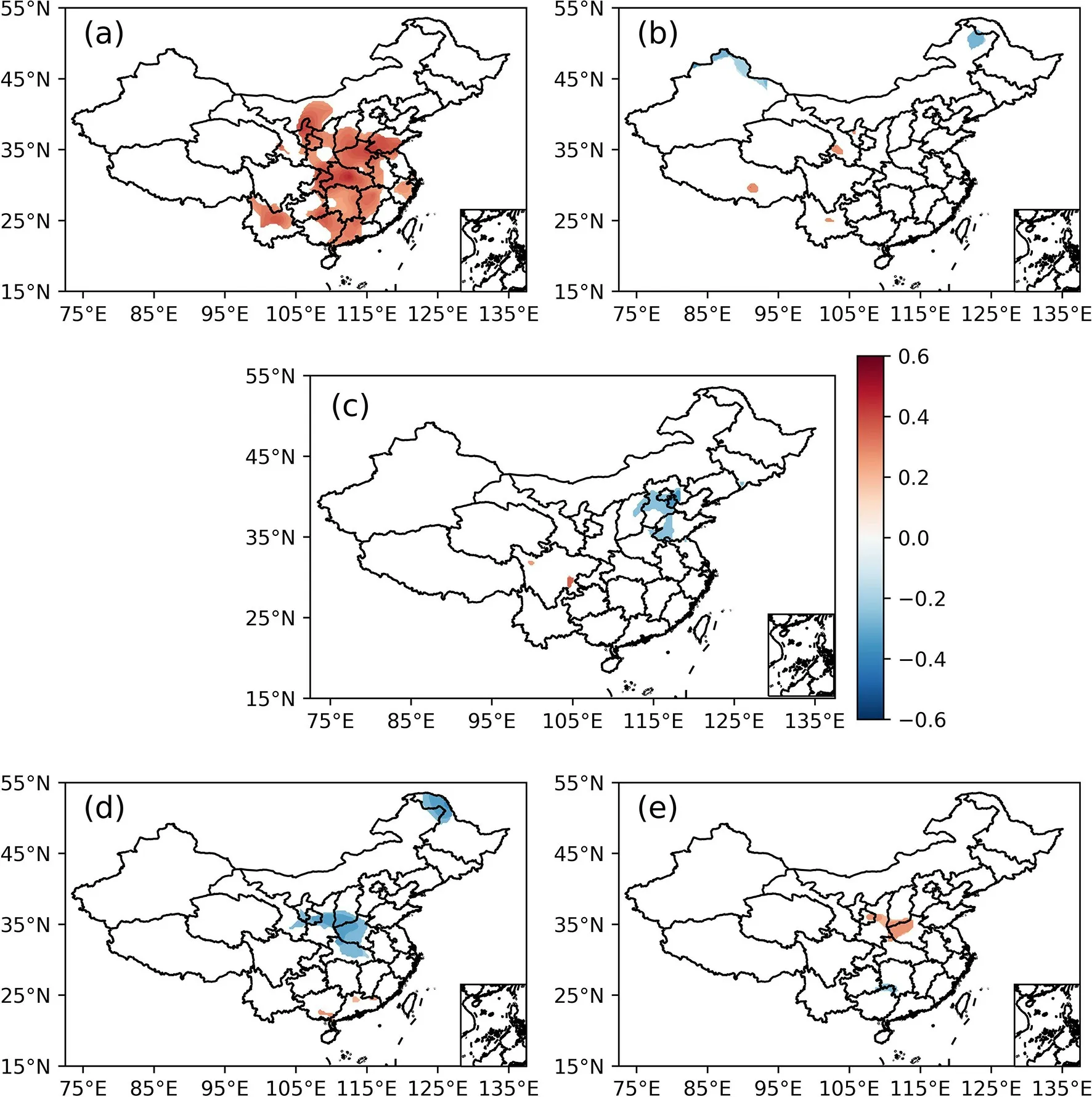
Fig. 6. Correlations between ACA intensity index in the Northern Hemisphere and precipitation at 160 stations in China in winter from 1951 to 2020. The shaded area is the significant-correlation area that passes the t-test at the α=0.05 level. (a) Iceland low. (b) North Atlantic High. (c) Mongolia High. (d) Aleutian Low. (e) North Pacific High.
By comparing Tables 2 and 3, it is reasonable and effective to test the significance of the correlation-coefficient field r of an example by using the EMC method and through the significant-correlation area.

Table 2. Area with significant correlations between ACA intensity indices and temperature/precipitation from 1951 to 2020 and the result of the EMC method test.

Table 3. The number of the stations with significant correlations between ACA intensity indices and temperature/precipitation from 1951 to 2020 and the result of Livezey method.
4. Conclusions
In summary, this paper analyzes the defects of the Livezey method for significance testing of a correlation-coef-ficient field r, constructs a new statistic(the significant-correlation area of r), and presents an EMC method for significance testing of r using. The Livezey method implies an assumption of the spatial independence of the correlationcoefficient field. In fact, the spatial distribution of the lattice or site network of the circulation and climate field is generally not uniform, and the field quantity on the adjacent lattice or site must have a certain correlation; otherwise, the system in the circulation and climate field cannot be given. The significance test by the EMC method can eliminate the influence of parent-space correlation. The significance test results from applying the method in this paper to the correlation chart r of the intensity index of ACAs in the Northern Hemisphere winter and the temperature and precipitation in China in the same period show that the test method in this paper is more reasonable than the Livezey method.
Acknowledgements.This work was supported by the National Key Research and Development Program of China (Grant No. 2018YFC1505602), the National Natural Science Foundation of China (Grant Nos. 41705055 and 41505088), the Project of Scientific Creation of Post-Graduates of Jiangsu (Grant No.CXZZ12_0485), the Creative Teams of Jiangsu Qinglan Project,and the Priority Academic Program Development of Jiangsu Higher Education Institutions (PAPD). The authors are very grateful for the constructive comments of two reviewers.
 Advances in Atmospheric Sciences2022年3期
- Advances in Atmospheric Sciences的其它文章
- Seasonal Prediction of Summer Precipitation over East Africa Using NUIST-CFS1.0
- Another Record: Ocean Warming Continues through 2021 despite La Niña Conditions
- A New X-band Weather Radar System with Distributed Phased-Array Front-ends: Development and Preliminary Observation Results
- A New Index Developed for Fast Diagnosis of Meteorological Roles in Ground-Level Ozone Variations
- Hydro-climatic Characteristics of Yarlung Zangbo River Basin since the Last Glacial Maximum
- Diagnosing SST Error Growth during ENSO Developing Phase in the BCC_CSM1.1(m) Prediction System
