Genetic diversity and relatedness inferred from microsatellite loci as a tool for broodstock management of fine flounder Paralichthys adspersus

Juliss J.Sánchez-Velásquez, Percy N.Pinedo-Bernl, Lorenzo E.Reyes-Flores,Crmen Yzásig-Brrer, Elin Zeld-Mázmel,＊

aLaboratory of Genetics, Physiology, and Reproduction, Faculty of Sciences, Universidad Nacional del Santa, Av Universitaria s/n, Nuevo Chimbote, 02712, Peru

bLaboratory of Mycology and Biotechnology, Universidad Nacional Agraria La Molina, Av.La Molina s/n, Lima, 12056, Peru

Keywords:

Fine flounder

Genetic diversity

Microsatellites

Paralichthys adspersus

Relatedness

A B S T R A C T

Paralichthys adspersus is a native species from the Pacific coast of South America that is of great economic importance for Peruvian aquaculture.Even though establishing sustainable farming depends on avoiding irreversible damage to the population gene pool due to processes such as inbreeding, studies focusing on genetically characterizing farmed stocks are yet to be documented.By using ten microsatellite loci on captive and wild individuals of P.adspersus, we successfully characterized the only commercial broodstock of this species in Peru by means of determining the genetic diversity and inferring relatedness.Although most microsatellite loci showed deviations from Hardy-Weinberg equilibrium, the genetic diversity levels in the commercial broodstock were considered healthy compared to those obtained for a wild population, with an average number of alleles of 17.40, an effective number of alleles of 9.14, and an observed and expected heterozygosity of 0.49 and 0.87.No significant differences between the broodstock and the wild population in terms of genetic diversity were observed.The fixation index and analysis of molecular variance also indicated a low rate of differentiation between both populations.In relatedness estimation, the analysis based on five method-of-moment estimators and a maximum-likelihood estimator showed the category “unrelated” as being the most probable relationship among the individuals within the commercial broodstock.Our findings reveal the conservation of genetic diversity in this population and outline potential breeding strategies that hatchery managers could use to minimize the loss of genetic diversity and long-term inbreeding.This could help establish proper genetic management in captive populations of P.adspersus and should apply to other captive stocks where pedigree information is lacking.

1.Introduction

Compared to the relatively stable trend in global capture fisheries,fish production through aquaculture is continually increasing as the demand for aquatic animals as food and for other uses intensifies and even surpasses some countries’ local capabilities (Harvey, Soto, Carolsfeld, Beveridge, & Bartley, 2017, FAO, 2020).To meet the current needs, stock enhancement has been implemented in several emerging species that, in addition to their biological and economic potential, have been shown to be culturally acceptable and reflect evolving consumer preferences (Harvey et al., 2017; Mylonas et al., 2019).For instance, in Peru, a country among the top ten countries with the largest aquaculture production in Latin America and the Caribbean (Wurmann, 2019), the highly prized flesh of the fine flounder,Paralichthys adspersus, has boosted its industrial farming since 2012 (PRODUCE, 2019).However,despite its remarkable growth over the last few years in terms of aquaculture production (PRODUCE, 2019), no science-based breeding program has yet been implemented to avoid the negative consequences of domestication.

A critical issue with domestication is the inability of most aquaculture centers to maintain high genetic diversity levels in the offspring populations (Jenkins, Ishengoma, & Rhode, 2020; Wellmann & Bennewitz, 2019).In the aquaculture industry, where most species are characterized by mass spawning and high fecundity, establishing a base population using only a few founders can be sufficient to produce large offspring populations for the market (Jenkins et al., 2020).However, if only a small number of individuals are used, the new population is likely to undergo a significant decrease in genetic diversity through a phenomenon known as founder effect, limiting the success of genetic improvement methods (Ghafouri-Kesbi, 2010; Kivisild, 2013).Loss of genetic diversity due to a founder effect has been observed in captive populations of largemouth bass,Micropterus salmoides(Wang et al.,2019); golden pompano,Trachinotus ovatus(Guo et al., 2018); Senegalese sole,Solea Senegalensis(Porta, Porta, Martínez-Rodríguez, &Alvarez, 2006); Atlantic salmon,Salmo salar(Skaala, Høyheim, Glover,& Dahle, 2004); and Japanese flounder,P.olivaceus(Liu, Chen, Li, & Li,2006; Sekino, Hara, & Taniguchi, 2003; Shikano, Shimada, & Suzuki,2008).In these studies, it has been shown that the participation of only a few breeders accompanied by poor reproductive management can result in a drop in genetic diversity by as much as 50% even in the first hatchery generation (Porta et al., 2006; Skaala et al., 2004).A signi ficant reduction in genetic diversity poses a serious problem since it can not only diminish the long-term response to selection but also increase the population homozygosity, affecting individual phenotypes and causing the population fitness to decrease (Trask et al., 2016; Wellmann& Bennewitz, 2019).The decline in fitness associated with an increase in inbreeding is called inbreeding depression, a phenomenon that should be avoided since it is correlated with reduced survival and increased disease susceptibility in inbred individuals (Ralls, Ballou, & Templeton,1988; Smallbone, van Oosterhout, & Cable, 2016).Therefore, preserving most of the initial population’s genetic diversity is of utmost importance for obtaining sustainable aquaculture productivity.

Maximal retention of genetic diversity can be achieved by establishing appropriate breeding programs such as selecting unrelated individuals to form the broodstock.For this, however, an accurate relatedness estimation is crucial.The most useful tools to estimate relatedness in fish populations are the molecular marker-based estimators developed by Wang (2002; 2007), Lynch and Ritland (1999), Ritland (1996), Li, Weeks, and Chakravarti (1993), and Queller and Goodnight (1989).These estimators evaluate the probability that two individuals share a randomly sampled allele; and even though they cannot determine a genuine relationship on the basis of coancestry, they can identify, assess, and prioritize the selection of breeding pairs with the lowest kinship rates (Gautschi et al., 2003).For example, using computer simulations, Ivy and Lacy (2012) and Fernández, Toro, and Caballero (2001, 2003) showed that the mean kinship method, consisting of selecting unrelated breeders to produce the offspring, allows minimizing inbreeding levels in the short and medium-term.Doyle,Perez-Enriquez, Takagi, and Taniguchi (2001) and Sekino, Sugaya,Hara, and Taniguchi (2004) also showed empirically that compared to a random mating scheme, the use of the minimal kinship criterion method enables the retention of most allelic diversity and heterozygosity in the offspring pools of red sea bream,Pagurus major, and Japanese flounder,P.olivaceus.Hence, relatedness estimation is a powerful tool for conserving genetic diversity by minimizing the population’s average kinship.

DNA markers such as microsatellites and the proliferation and refinement of statistical analyses are among the most important tools to estimate relatedness.Microsatellites are tandem repeats of short genetic elements (about 2-10 bp) that enable the retrospective assignment of an individual to family groups in the absence of physical labels or pedigree information (Press, Carlson, & Queitsch, 2014).The discriminating power of microsatellites relies on two essential features: high polymorphism and codominance (Castro et al., 2006; Jones, Small, Paczolt,& Ratterman, 2010; Norris, Bradley, & Cunningham, 2000).The high polymorphism of microsatellites, due to their high mutation rate, allows the existence of many alleles at a single locus, allowing more precise genetic comparisons and accurate kinship assignments (Castro et al.,2006; Norris et al., 2000).Likewise, their codominance allows rapid genotypification by enabling heterozygote individuals’ distinction from homozygote individuals (Webster & Reichart, 2005).Despite their high discriminating power, one practical drawback of microsatellites is that their application requires sequence information regarding the repeat motif priming sites; however, obtaining this information involves a process that is generally expensive and time-consuming (Rico, Rico, &Hewitt, 1996).Nevertheless, their transferability or cross-species amplification property allows utilizing microsatellite loci between phylogenetically close species, reducing the costs when researchers work on taxa with very low microsatellite frequencies or from which microsatellites are challenging to isolate (Oliveira, Pádua, Zucchi,Vencovsky, & Vieira, 2006).Because no microsatellite loci have been described forP.adspersusto date, this last property means that the freely available flanking microsatellite primers developed for the genusParalichthyscan be used inP.adspersus.

In this article, we present the genetic characterization of the only commercial broodstock of the fine flounder,P.adspersus, in Peru based on ten microsatellite loci.First, we aimed to assess the maintenance or loss of genetic diversity in the commercial broodstock by comparing its genetic diversity levels with those found in a wild population.The second goal was to infer patterns of relatedness to provide hatchery guidelines for sustainable broodstock management in order to conserve most of the initial population genetic diversity and avoid the generation of inbred individuals in ensuing generations ofP.adspersus.

2.Materials and methods

2.1.Sampling areas and DNA extraction

Caudal fin tissue of 70 live adults ofP.adspersusbelonging to a hatchery population formed by wild captives and domesticated broodstocks was provided by an aquaculture center located in Ancash, Peru, in 2015.The collected individuals had a body weight and size of 1953.96±97.61 g and 50.11 ±0.76 cm on average.Caudal fin tissue was selected so as to not compromise the survival and swimming performance of live individuals (Champagne, Austin, Jelks, & Jordan, 2008).Caudal fin tissue of wild individuals from the central north and south coasts of Peru (Ancash and Tacna), with approximate body weight and size of 2139.67 ± 317.94 g and 52.82 ± 2.09 cm on average, was also collected between 2015 and 2016.Wild individuals consisted of 12 individuals from Gramita Beach, 18 individuals from Culebras Beach, six individuals from Vila Vila Beach, and six individuals from Morro Sama Beach (Fig.1).Given that the focus of the present study was on evaluating the status of a hatchery broodstock by comparing its genetic diversity with that of a wild reference stock, wild individuals from Ancash and Tacna were analyzed as a single population.Total genomic DNA was extracted from approximately 20 mg of tail fin tissue using the SDS-proteinase K/phenol-chloroform digestion method adapted from Taggart, Hynes, Prodöuhl, and Ferguson (1992) and stored at -20 ℃.The DNA concentration of each sample was assessed using the Epoch microplate spectrophotometer (BioTek Instruments, Vermont, USA);afterward, the concentration was adjusted to 25 ng/μL.

Fig.1.Map showing the five sampling locations of Paralichthys adspersus in Peru.PDF: Aquaculture center.

2.2.Microsatellite genotyping and data analysis

Genetic diversity was evaluated using the flanking primers of ten dinucleotide microsatellite loci developed forP.olivaceus.They includedPoli2TUF,Poli9TUF,Poli23TUF,Poli28TUF(Coimbra et al., 2001),Po35,Po56,Po91(Sekino & Hara, 2001),KOP45,KOP51(Kim et al., 2009),andPol-4(Takagi, Yoshida, & Taniguchi, 1999) loci, which showed the highest polymorphism and heterozygosity when applied to population studies in this species.Only dinucleotide repeats were chosen because they are reported to have the highest mutation rate compared to any other type of repeat (Di Rienzo et al., 1994; Kruglyak, Durrett, Schug, &Aquadro, 1998).The PCR reactions were performed in a total volume of 7 μL reaction mixture containing 4.32 μL PCR water, 0.66 μL Taq Buffer KCl-MgCl2(10X), 0.51 μL MgCl2(25 mM), 0.33 μL dNTPs (2.5 mM),0.06 μL forward/reverse primer (12.5 μM each), 0.06 μL Maximo Taq DNA Polymerase (5 U/μL) (GeneON, Deutschland, Germany), and 1 μL DNA (25 ng/μL).Annealing temperature (Ta), denaturation, annealing,elongation times, and the number of cycles for each locus are detailed in Table S1.PCR amplification products were verified on 2% agarose gel and genotyped by means of capillary electrophoresis using a Fragment Analyzer™ Automated CE System (Advanced Analytical Technologies,Inc., Iowa, USA) and a DNF-900 dsDNA Reagent Kit (Advanced Analytical Technologies).Allele scoring was performed using PROSize data analysis software (Advanced Analytical Technologies) by interpolating their position to molecular weight markers and DNA ladders(35-500 bp DNA Marker and 75-400 bp Range DNA Ladder, both from Advanced Analytical Technologies).

Stuttering, allelic dropout, typographic errors, and the presence of null alleles were evaluated using Micro-Checker v.2.2.3 (Van Oosterhout, Hutchinson, Wills, & Shipley, 2004).The frequency of null alleles was calculated using ML-Null Freq v.1.0 (Kalinowski & Taper, 2006).The Hardy-Weinberg equilibrium (HWE) for each locus in each population was tested using Genepop v.4.2 (Rousset, 2008).The significance level for each HWE test was assessed by employing a Markov chain Monte Carlo (MCMC) procedure with 1000 dememorizations, 100 batches, and 1000 iterations per batch (Holm, 1979).The polymorphic information content (PIC) at each locus was determined using CERVUS v.3.0.7 (Kalinowski, Taper, & Marshall, 2007).Allelic richness (R) was evaluated using HP-Rare v.1.0 (Kalinowski, 2005).The diversity for each locus was quantified as the number of alleles per locus (A), the effective number of alleles (ae), allelic frequency, and observed and expected heterozygosity (Ho, He) using GenAlEx v.6.5 (Peakall &Smouse, 2012).For all genetic diversity measures, the mean and the standard error of the mean (SEM) are shown.Statistical differences between the genetic diversity measures found in the captive and wild populations were tested using Student’s t-tests on GraphPad Prism v.7.0.Pvalues＜0.05 were considered to be statistically significant.

2.2.1.Population structure and genetic differentiation

To determine population structure and genetic differentiation, the fixation index (FST) was calculated and analysis of molecular variance(AMOVA) as a function of allele frequencies performed in ARLEQUIN v.3.5 (Excoffier & Lischer, 2010).Statistical significance for both analyses was examined using 10 000 permutations.To analyze the FSTvalues, the definition proposed by Wright (1978) was used, where values of 0-0.05, 0.05-0.15, 0.15-0.25, and＞0.25 indicate little, moderate,great, and very great genetic differentiation, respectively.

2.2.2.Patterns of relatedness

The information content of each locus was measured by calculating the informativeness for relationship (IR) and informativeness for relatedness (Ir) using KinInfor v.2.0 (Wang, 2006).IRmeasures the information content of a microsatellite locus for discriminating different relationship categories, and Iris the amount of information a microsatellite locus provides for estimating relatedness (Wang, 2006).IRand Irwere calculated for three hypothetical kinship assumptions.The primary and null hypotheses for each assumption were as follows: (i)full-sibs (FS) and unrelated (UR), (ii) half-sibs (HS) and UR, and (iii) FS and HS.In all assumptions, 1 000 000 dyads were simulated, assuming a prior Dirichlet distribution (1,1,1).The significance level was set at 0.05 with a precision level of 0.01.The power for relationship inference(PWr) of the ten microsatellite loci was also determined through an iterative approach (Kozfkay et al., 2008).In this approach, the first round included the highest-ranked locus, the second round included the two highest-ranked loci, the third round included the three highest-ranked loci (all according to IR, Ir, and PWr), and so on until the power of all loci was evaluated.

Because choosing the best marker-based relatedness estimator is necessary for performing kinship assignments with a robust statistical framework, we estimated the coefficient of relatedness (rxy) using five method-of-moment estimators: LynchRdrLR(Lynch & Ritland, 1999),RitlandrR(Ritland, 1996), LynchLirLL(Li et al., 1993), QuellerGTrQG(Queller & Goodnight, 1989), and WangrW(Wang, 2002) using COANCESTRY v.1.2.1 (Wang, 2011).It is important to highlight that although these estimators were developed from the identical by descent(IBD)-based concept of relatedness, whererxycan only go from 0 to 1 if neither of the two individuals being compared is inbred, these estimators can give negativerxyvalues if the average relatedness among sampled individuals becomes close to zero (Wang, 2014, 2017).However, these values have biological meaning if they are understood as the correlation of homologous genes between and within individuals due to shared ancestry, as conceived in the original correlation concept of relatedness (Wang, 2014; Wright, 1921).This means that if negative values are found, the individuals are less related in ancestry than the average-i.e., they have genotypes less similar in expectation than the average (Wang, 2014).Because the method-of-moment estimators can give negative values if the average relatedness among sampled individuals becomes close to zero, the final relationship estimation among a pair of individuals was established as the consensus between each method-of-moment estimator and a maximum-likelihood (ML)method, whererxyis constrained in the legitimate range of [0,1] based on the IBD concept (Wang, 2014).The ML estimates of pairwise relatedness between individuals were determined through ML-Relate v.1.0(Kalinowski, Wagner, & Taper, 2006).

The cutoff value used to group the formed dyads in the different relationship categories was established following the suggestion of Blouin, Parsons, Lacaille, and Lotz (1996) since our dataset did not include pedigree information.According to these authors,parent-offspring (PO), FS, HS, and UR dyads can be distinguished using the midpoint between the meanrxyvalues of any two distributions.To calculate therxyof each category, genealogical relationships between individuals are conveniently represented mathematically as probabilities that genotypes in the individuals share zero, one, or two alleles IBD(Kalinowski et al., 2006).Following this definition, if we letk0,k1, andk2represent the probabilities that two individuals share zero, one, or two alleles at a locus if two individuals are PO, all loci will share one allele (k0=0,k1=1,k2=0).If two individuals are FS, loci may share 0,1, or 2 alleles (k0=0.25,k1=0.5,k2=0.25).If two individuals are HS,loci may share 0 or 1 allele (k0=0.5,k1=0.5,k2=0).If two individuals are UR, all loci within the pair of individuals will have no alleles (k0=1,k1=0,k2=0) (Kalinowski et al., 2006; Wagner, Creel, & Kalinowski,2006).Using thesek-coefficients and assuming that neither of the two individuals being compared is inbred, the relationship betweenk-coefficients andrxyis defined as:

Applying this formula, therxyvalues for PO, FS, HS, and UR would be 0.5, 0.5, 0.25, and 0, respectively.Following the suggestion of Blouin and colleagues, if we want to distinguish between FS and HS, the dyad falling to the right of the cutoff value of 0.375 (halfway between 0.25 and 0.5) would be classified as belonging to the FS category.Using this strategy to group all dyads, FS were the dyads with anrxybetween 0.375 and 0.5, HF the dyads with anrxybetween 0.375 and 0.125, and UR the dyads with anrxylower than 0.125.

Although it has been shown that the midpoint between the mean values of any two distributions places most dyads in their real categories(Borrell et al., 2004), when analyzing real and virtual descendent,Borrell et al.(2004) demonstrated that between 71% and 100% dyads exhibiting anrxylower or equal to zero were correctly identified as UR individuals.Thus, we used zero as the cutoff point to distinguish UR individuals instead of 0.125.

The probability that a dyad of one type of relationship would be misclassified as belonging to another type of relationship was calculated as type I and II errors using the midpoint of the means of two adjacent relatedness distributions as the assignment threshold (Kozfkay et al.,2008).The percentage of HS falling to the right of the assignment threshold between HS and FS and the percentage of UR falling to the right of the assignment threshold between UR and HS were determined as the expected type I error rate (unrelated individuals classified as related).The percentage of FS falling to the left of the assignment threshold between HS and FS and the percentage of HS falling to the left of the assignment threshold between UR and HS were denoted as the type II error rate (related individuals classified in a less related category).

3.Results

3.1.Genetic diversity

The captive and wild populations ofP.adspersuswere successfully genotyped at ten microsatellite loci (Table 1).In the captive population,no microsatellite loci showed HWE, whereas only two loci (Po91andKOP51) were at equilibrium in the wild population.The absence of HWE in most loci was supported by analysis of the expected distribution of heterozygotes at each locus, which suggested the presence of null alleles in both populations.The mean PIC value in the captive population was 0.86 ±0.02, with values ranging from 0.74 forPoli2TUFto 0.93 forPo56.The average numbers of A and R were 17.40 ± 2.02 and 12.50 ±1.18.For both parameters, thePoli23TUFandPo91loci showed the lowest and highest values.The average value of aewas 9.14 ±1.20 and ranged between 4.40 forPoli2TUFand 14.14 forPo91.The average value of He through all loci was 0.87 ±0.02, while that of Ho was 0.49±0.06 (57% lower than He).By locus, the value of Ho ranged between 0.23 forPoli2TUFand 0.73 forPol-4, withPo91,Pol-4,KOP45, andPo56being the loci showing the most homogeneous values between He and Ho.Within the captive population, when the genetic diversity between males and females was compared, we also found no significant differences, except for the number of alleles due to the great difference in sample size between the two groups (Table S2).

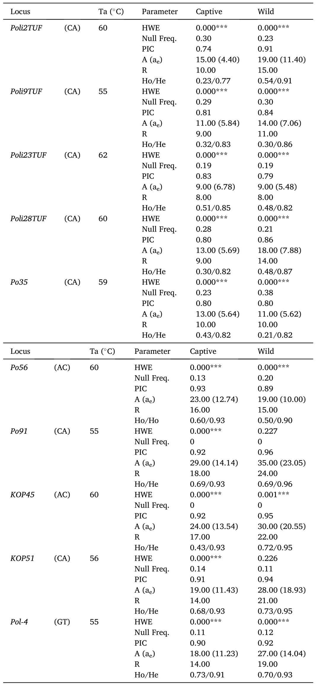
Table 1Genetic diversity in the captive and wild population of Paralichthys adspersus based on ten microsatellite loci.Repeat motif, annealing temperature (Ta), Hardy-Weinberg equilibrium (HWE), frequency of null alleles,polymorphic information content (PIC), number of alleles per locus (A), effective number of alleles (ae), allelic richness (R), and observed and expected heterozygosity (Ho/He) are shown.

In the wild population, the average PIC value was 0.89 ±0.02, with values ranging from 0.79 forPoli23TUFto 0.96 forPo91.The average values of A and R were 21.00 ± 2.73 and 15.90 ± 1.72 (19% and 25% higher than the values registered in the captive population).The average value of ae was 12.41 ±2.04 and, it ranged between 5.48 forPoli23TUFand 23.05 forPo91.For He and Ho, the average values were 0.90 ±0.02 and 0.54 ±0.06, respectively.Compared to the captive population, the value of Ho indicated the presence of 9.25% more heterozygosity in the wild population.By locus, the Ho value ranged from 0.21 forPo35to 0.73 forKOP51, withPo91,KOP45,Poli2TUF,Pol-4,KOP51, andPo56being the loci with the most homogeneous values between He and Ho.Although the different diversity measures were higher in the wild population, they were not significantly different from those registered in the captive population.

Regarding the distribution of allelic frequencies, rare alleles (alleles at frequencies lower than 0.10, Thomson, Cooch, & Conroy, 2009) were detected at all loci and without association with a particular locus in any population (Fig.S1).Population-wise, our results indicated the presence of 79% of rare alleles in the captive population and 88% of alleles at the same frequencies in the wild population.

3.2.Population structure and genetic differentiation

The FSTpresented a value of 0.024 (P≥0.001), indicating that 97.6% of the variance in allelic frequencies was due to intrapopulation genetic variation.The AMOVA also showed that variation within individuals was the main source of genetic variation (Table 2).The analysis of alleles shared between individuals from the captive population and the two wild subpopulations (individuals collected from Ancash and Tacna) also demonstrated the degree of similarity between samples.The analysis revealed that wild individuals collected from Ancash and the captive population shared 65% of alleles.Likewise, wild individuals collected from Tacna and the captive population shared 46% of alleles.Thus, the high proportion of alleles shared by the captive and wild populations showed that neither population had alleles at a proportion significantly higher or lower to distinguish it as a population genetically different from the others.

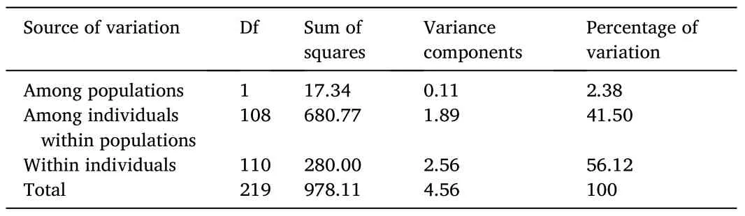
Table 2Summary of the analysis of molecular variance (AMOVA).The data shows interpopulation and intrapopulation variation between the captive and wild population of Paralichthys adspersus.

3.3.Relatedness estimation

Among the ten microsatellite loci, thePo91andPoli2TUFloci ranked as the highest and lowest in terms of information content for relatedness estimation when the three hypothetical relationships were assumed(Table S3).The simulated power in differentiating FS from UR individuals ranged from 0.50, when the highest-ranked locus was evaluated alone, to 0.99, when all ten loci were evaluated (Fig.2).The simulated power in differentiating HS from UR individuals ranged from 0.26 to 0.77, and the simulated power in differentiating FS from HS ranged from 0.30 to 0.76 (Fig.2).

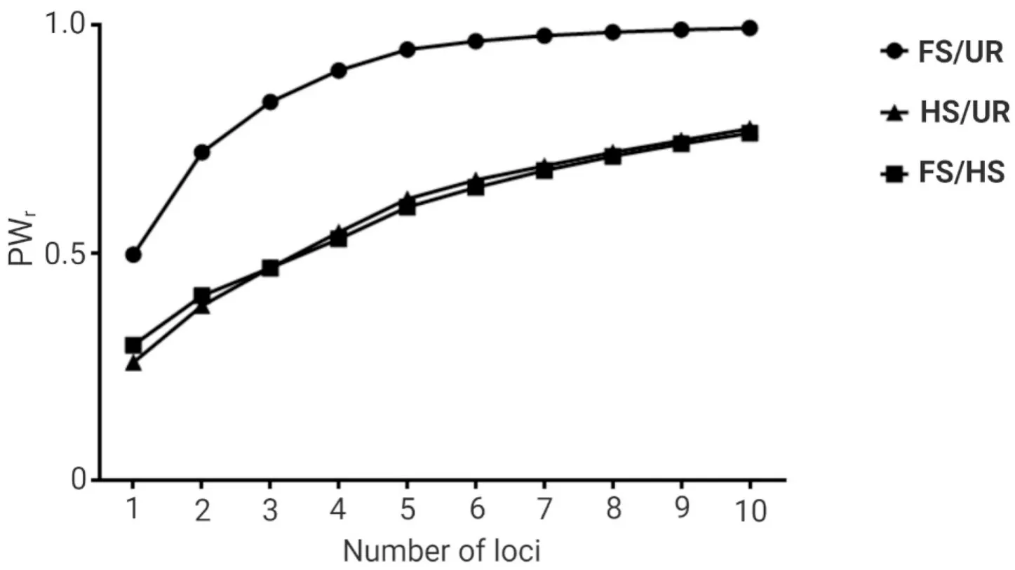
Fig.2.Power for relationship inference (PWr) utilizing different numbers of microsatellite loci in the captive population of Paralichthys adspersus.The power for relationship inference was obtained using the KinInfor program simulating 1 000 000 dyads for three hypothetical relationships: (i) full-sibs and unrelated (FS/UR), (ii) half-sibs and unrelated (HS/UR), and (iii) full-sibs and half-sibs (FS/HS).The first data point corresponds to the PWr for the simulation utilizing the highest-ranked locus alone,the second data point corresponds to that utilizing the two highest-ranked loci, and so on until all loci were evaluated.

The average values forrxyin all relatedness estimators supported the category “unrelated” as the most probable type of relationship between the individuals comprising the captive population ofP.adspersus(Table 3).The values forrxyranged from -0.015 for therLR/rQGestimators to 0.065 for therMLestimator.The data also indicated an overlap in the range of values between two adjacent relatedness categories.Among all relatedness estimators, therWestimator presented the lowest fraction of FS misclassified as HS, and with therLLestimator, one of the lowest fractions of HS misclassified as UR.For the type I error rate, therLRestimator showed the lowest fraction of HS misclassified as FS and the lowest fraction of UR misclassified as HS.By contrast, therQGandrLRestimators showed the highest fraction of FS misclassified as HS and HS pairs misclassified as UR, respectively.TherQGandrLLestimators also showed the highest fraction of HS misclassified as FS, and UR pairs misclassified as HS (Table 4).Considering these results, using therWandrLLestimators, aquaculture managers could select unrelated individuals with high precision by eliminating type II errors-i.e., avoiding the selection of related individuals as mating pairs.As both estimatorsrWandrLLpresented the lowest type II error rates, the final consensus outcome from COANCESTRY and ML-Relate is only reported for these estimators(Table S4).In the final matrix, when crossing the 14 females and 46 males forming part of the captive population, we obtained 644 possible interactions.The calculated relatedness indicated 93.79% recommended crosses (among UR pairs), 5.59% marginal crosses (among HS pairs), and 0.62% inadmissible crosses (among FS pairs).

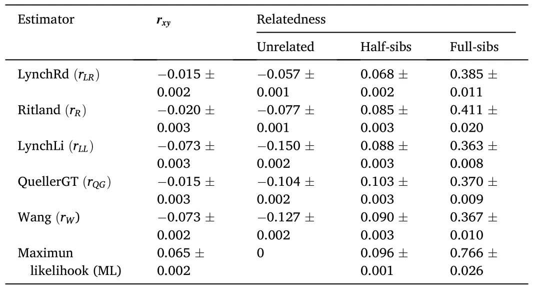
Table 3Average relatedness coefficient (rxy) in the captive population of Paralichthys adspersus calculated from six relatedness estimators.The average value and standard error of the mean for each estimator are shown.

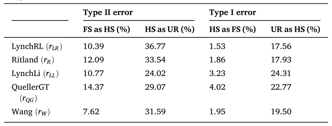
Table 4Proportion of misclassified dyads among two adjacent relatedness categories.Type II and I error rates for the five method-of-moment estimators were calculated using the midpoint of the means of two relatedness distributions as the assignment threshold.

4.Discussion

The sustainable improvement of aquaculture’s genetic resources depends on the conservation of genetic diversity-the source for adaptation to the changing environmental conditions and long-term response to selection (Wellmann & Bennewitz, 2019).In the present study, all microsatellite loci in the commercial broodstock ofP.adspersusand 8 out of the 10 loci in the wild population showed deviations from HW expectations.Consistent with our findings, Sekino, Hara, and Taniguchi(2002), Zeinab, Shabany, and Kolangi-Miandare (2014), and Napora-Rutkowski et al.(2017) showed that deviations from HWE are relatively common in captive populations since hatchery managers form fish stocks utilizing a limited number of founding individuals and an unequal sex ratio.In the wild population, the genetic imbalance in 8 out of the 10 microsatellite loci might have resulted from inbreeding, null alleles,ecological events, or a Wahlund effect (Karlsson & Mork, 2005;Sahyoun, Guidetti, Franco, & Planes, 2016).Among these possibilities,inbreeding can be ruled out since, for this, the wild population would have undergone a reduction in the effective population size to the point where inbreeding became significant-an unlikely event unless it could be shown that there was strong selective mating (Hoarau, Rijnsdorp,Van Der Veer, Stam, & Olsen, 2002).Another possibility is the presence of null alleles, frequently detected in the order Pleuronectiformes due to the low conservation of microsatellite flanking regions (Castro et al.,2006).Because at frequencies greater than 0.2 (values found in 5 out of the 10 microsatellite loci used in this study), null alleles can result in genotypes apparently inconsistent with classical Mendelian inheritance(Dakin & Avise, 2004), null alleles could be the most likely explanation for the absence of HWE in the wild population.However, they are unlikely to be the only reason (Ruzzante, Taggart, & Cook, 1996).Indeed,although theKOP45locus had no null alleles, it deviated from HWE.By contrast, although theKOP51locus presented null alleles, a deviation from HWE was not observed.Therefore, other processes, such as ecological events or a Wahlund effect, could explain the absence of HWE in this population (Karlsson & Mork, 2005; Sahyoun et al., 2016).In terms of an ecological event, the wild population could have consisted of large populations that were historically in contact but are currently isolated and fixed for different alleles at equilibrium (Neigel, 2002).If this were the case, a deviation from HWE is expected if the time required to approach this equilibrium is greater than most individuals’ age(Neigel, 2002).Another possibility is a Wahlund effect, which could have occurred if there was a physical merging of populations with different allelic frequencies into a single population.Future studies utilizing individuals from other localities along the coasts of Peru and the sampling of more than 25 individuals-sample size recommended to detect the most informative alleles for assessing genetic structure (Hale,Burg, & Steeves, 2012)-are still necessary to explain whether there was a substructure, merging of populations, or if the deviations from HWE can only be explained by the presence of null alleles.

Lack of genetic structure among wild populations inhabiting the South Pacific was reported in several studies includingCancer setosus,Dosidicus gigas,Trachurus murphyi, andScomber japonicus(Barahona,Oré-Chávez, & Bazán, 2017; Cárdenas et al., 2009; Gomez-Uchida,Weetman, Hauser, Galleguillos, & Retamal, 2003; Marcelo-Ibá˜nez &Poulin, 2014).The effect of ocean currents facilitating genetic exchanges among subpopulations was noted in these studies, but there are limited reports on their effect on population genetic structure patterns of demersal species such asP.adspersus.In the present study, we found significant differences in neither allelic richness nor heterozygosity when we compared genetic diversity between the Central Northern and Southern wild subpopulations ofP.adspersus(Table S5).Moreover, the AMOVA andFSTrevealed no genetic differentiation between the two groups (0% and -0.002) (Table S6).This genetic homogeneity inP.adspersushas also been documented in otherParalichthysspecies.For example, using 11 microsatellite loci, Sekino and Hara (2001) showed that the Japanese populations ofP.olivaceuslack genetic structure across the 3000 km of the Japanese coast facing the Sea of Japan, a region with a geographic area that almost equals the Peruvian coast.The genetic homogeneity inP.olivaceushas been attributed to the passive larval dispersion by oceanic currents, which may homogenize genetic compositions even when the extent of adult movements seems to be limited.Although the mode and extent of larvae dispersal in the Pacific Ocean forP.adspersusis not clear, it can be assumed that the Humboldt Current System (HCS), extending along the west coast of South America(Thiel et al., 2007), might be effectively mixing genetic components among these populations.Indeed, Gomez-Uchida et al.(2003), Marcelo-Ibá˜nez and Poulin (2014), Cárdenas et al.(2009), and Barahona et al.(2017) proposed that the occurrence of large-scale gene flow displayed by many marine species present in the South Pacific could reflect the effect of the HCS and oceanographic flows, which would allow effective mixing of populations in an asymmetric bidirectional way along the South Pacific Sea (Barahona et al., 2017).Considering thatP.adspersushas a planktonic stage that lasts as long as 60 days (Silva & Oliva, 2010),similar toP.olivaceus, it is highly likely that the long planktonic stage,along with the effect of the HCS and lack of oceanographic barriers,creates high levels of larval dispersion and, therefore, the observed genetic homogeneity among local populations.However, we should mention that these results constitute a preliminary observation.Further analyses with greater sample sizes and more sampling locations are needed in order to determine whether the homogeneity of molecular variance among wild subpopulations extends along the Peruvian coast and whether those subpopulations should be treated as a single panmictic population.The accumulation of biological and ecological data such as migration rates will also be crucial (Sekino & Hara, 2001).If high levels of migration among populations are found, they could explain the apparent high gene flow among wild subpopulations ofP.adspersus.

One of the major objectives of this study was to assess the maintenance or loss of genetic diversity in the commercial broodstock ofP.adspersusby comparing its genetic diversity levels with those found in a wild population.Our results revealed no significant differences between the captive and wild populations in terms of heterozygosity.Although the difference in sample size between these populations (70 and 40 individuals, respectively) could suggest bias in heterozygosity estimation, it can be reliably inferred that the heterozygosity levels are similar since the precision of heterozygosity estimation does not increase significantly beyond a sample size of 25 individuals if highly polymorphic loci are examined (Hale et al., 2012; Nei, 1978; Pruett &Winker, 2008).This conservation of genetic diversity in terms of heterozygosity is not surprising since high levels of heterozygosity and even excess can be found in captive populations if they were established using heterozygous founders (Sekino et al., 2003).Indeed, in captive populations ofS.salarandS.maximus, Norris, Bradley, and Cunningham(1999) and Coughlan et al.(1998) reported the conservation of heterozygosity despite a significant decrease in allelic diversity.However, it is important to note that although heterozygosity is proportional to the amount of genetic variance at a locus (Allendorf, 1986), it is relatively insensitive to the genetic changes that could occur in captive populations within the first generations of isolation (Allendorf, 1986;Hedgecock & Sly, 1990).For example, despite the fact that only a small fraction of the initial heterozygosity is expected to be lost due to small bottlenecks, such bottlenecks have a major effect on other diversity parameters such as allelic diversity measures (Allendorf, 1986; Caballero & García-Dorado, 2013).In fact, compared to heterozygosity, the captive population showed a more pronounced loss of the number of alleles, allelic richness, and effective number of alleles at a rate of allele loss observed in other captive populations such asS.salar(Koljonen,Tähtinen, Säisä, & Koskiniemi, 2002; Verspoor, 1988).Therefore,although the lack of knowledge about the origin of the F1individuals forming part of the captive population makes it impossible to assess the magnitude of the reduction in genetic diversity, our results showed that allelic diversity could strongly decrease after artificial selection, which can be followed by a significant loss of heterozygosis if the selective pressure increases (Sekino et al., 2002).

Even though there was a general trend toward the loss of genetic diversity in the captive population ofP.adspersus, we did not find significant differences among its genetic diversity levels and those found in a wild population.The AMOVA andFSTresults also indicated low levels of genetic differentiation between both populations.This shows that the captive population constitutes a good broodstock to maintain high genetic diversity levels in offspring populations if appropriate breeding schemes are established.Minimizing the populations’ global coancestry and long-term inbreeding provides an ideal approach for this purpose(Doyle et al., 2001; Sekino et al., 2002).In this study, by analyzing relatedness, we found that most individuals within the broodstock were categorized as unrelated, a result that should be interpreted with caution as the degree of discrimination between the different relatedness categories depends on the number of microsatellite loci being used (Blouin et al., 1996).For instance, while 10 microsatellite loci provide 87% accuracy for relatedness estimation compared to a kinship assignment using pedigree information, 24 microsatellites provide 97% accuracy(Wagner et al., 2006).Nonetheless, although increasing the number of microsatellite loci improves relatedness classification, the use of at least eight highly variable microsatellite loci with a stricter decision criterion(avoiding the type II error rate) discriminates related and unrelated pairs in the same measure (Norris et al., 2000).Hence, our relatedness estimation using ten microsatellite loci allows choosing potential unrelated mating pairs with high precision.

Another critical parameter to estimate relatedness is selecting microsatellite loci with the highest informativeness levels to increase the estimation’s accuracy and reduce the genotyping costs and efforts(Wang, 2006).One efficient approach to achieving this is choosing the lowest number of highly ranked loci on the basis of their power for relationship inference.In this study,five of the highest-ranked loci already provided more than 90% power in differentiating FS from UR pairs; however, it was necessary to use ten microsatellite loci in order to gain about 80% power for differentiating HS from UR pairs and FS from HS pairs.This means that if the aquaculture center’s goal is a rapid distinction of related pairs from unrelated pairs, this estimation could be performed utilizing only the five highest-ranked loci.If obtaining a greater level of accuracy is needed, especially to discriminate HS from UR, then the use of more loci is advised.Another critical parameter to take into account when inferring relatedness is the type II error rate since the cost of an incorrect inclusion (crossing individuals as if they were unrelated when they are not) could be higher than the cost of an erroneous exclusion (deciding not to breed animals that are actually unrelated) (Willis, 1993).In this study, therWandrLLestimators showed the lowest type II error rates, a result that agrees with the findings obtained by Wang (2002, 2017), who demonstrated that compared to other relatedness estimators, therWandrLLestimates tend to be unbiased irrespective of the sample size and actual relationship.Moreover,the estimator’s sampling variances for therWestimator consistently diminish with an increasing number of alleles per locus, resulting in increased accuracy if polymorphic loci are used (Wang, 2002).Nevertheless, the relatedness estimator’s final choice will depend on the type of error rate the breeding program wants to minimize.For example, if managers want to exclude HS or FS, the best approach would be to choose the estimator with the lowest type II error rate despite there being a larger type I error rate.

Importantly, how small or large the type I or II error rates are depends on the cutoff values used to discriminate among the different relatedness categories.For example, applying the average value between two adjacent categories as a cutoff point allows obtaining bias values similar to those reported using samples with known kinship(Borrell et al., 2004; Guan et al., 2016; Kozfkay et al., 2008).However,when assigning this value as a cutoff point to discriminate unrelated individuals, there is a high risk of incorrectly assigning HS to a less related category.For instance, inP.olivaceus, Sekino et al.(2004)showed that when the mean value for UR dyads is applied as a cutoff value, 3 out of 10 HS are still incorrectly classified as UR.Instead, when using zero as the cutoff to identify UR pairs, only 1 in 10 cousins and only 1 in 100 HS are classified as UR pairs (Norris et al., 2000).Borrell et al.(2004) also indicated that UR individuals could be identified with a confidence of 80% if zero is used as the cutoff value.Because we utilized zero as the cutoff point to distinguish HS from UR pairs, our data allow us to design an efficient reproductive system whose primary objective will be to avoid mating among closely related individuals.Although the application of such methods will not necessarily eliminate inbreeding,they will improve the retention of genetic diversity in the ensuing captive populations ofP.adspersus.

It is important to highlight that regardless of the estimator and cutoff value used, low polymorphism levels are among the principal constraints for achieving an accurate relatedness estimation.When the markers’ polymorphism is low, even if a large number of loci are used,the genetic discrimination between related and unrelated individuals is significantly affected (Taylor, 2015).For instance, in captive populations ofS.salar, Norris et al.(2000) showed that increasing the number of microsatellite loci from four to eight results in very little additional discrimination if the four additional markers exhibit low polymorphism.Another important feature to take into account is the presence of null alleles.When the frequency of null alleles exceeds 0.20,the assignment errors can underestimate the exclusion probabilities and be responsible for about 1.4% of the differences between theoretic kinship allocations and those obtained when considering a real situation(Borrell et al., 2004; Dakin & Avise, 2004).Therefore, the level of confidence in relatedness estimation will strongly depend on the type of microsatellite loci the researcher decides to use.

Besides minimizing kinship levels, it is important to highlight that to conserve genetic diversity, an unbiased sex ratio should also be used.It has been shown that as the sex ratio deviates from 1:1 in either direction(males or females), the ratio effective population to census size (Ne/N)declines (Briton, Nurthen, Briscoe, & Frankham, 1994).Indeed, if we apply the formula proposed by Wright in 1933 (Wang, Santiago, & Caballero, 2016), the commercial broodstock ofP.adspersus, with a male-biased sex ratio of 3 to 1, would be expected to have an Ne of only 45 compared to the total population size if an equal sex ratio is utilized.A reduction in the Ne could in turn affect the establishment of sustainable aquaculture management by diminishing the efficacy of selection(Charlesworth, 2009).Briton et al.(1994) also found that all measures of genetic variation, such as the polymorphisms levels, average gene diversity, and average number of alleles per locus, are reduced if a biased sex ratio is utilized.Using simulations of successive generations based on allelic data, Çiftçi, Yelmen, De˘girmenci, and Kaya (2020) also showed that when the mating strategy includes a biased sex ratio, fewer alleles survive over generations, and the genetic diversity drops faster.This is worrisome since although only unrelated individuals from the current broodstock ofP.adspersusare crossed in order to maintain the genetic diversity levels, mating among relatives will be inevitable if those new offspring populations are used as broodstock in the future.Although the general conclusion from these observations is to avoid a mating strategy that includes a biased sex ratio, this recommendation is not always applied or possible for most aquaculture centers.If a biased sex ratio must be used, then it is advisable to keep the lowest sex ratio possible and replace male and female individuals as frequently as possible, e.g., generating an offspring population utilizing one male and five females will be much better than a population formed utilizing a single male and ten females (Ne of 6.6 versus 3.6) (Briton et al., 1994).

5.Conclusions

Genetic gain through the selection of phenotypically superior individuals is a primary goal for aquaculture centers.However, a few and closely related individuals are usually selected to form the new populations during the process.Such practices hinder sustainable farming since they reduce genetic diversity, which is critical for maintaining the population’s fitness.Balancing the hatchery’s goals with the conservation of genetic diversity, therefore, remains a challenge.Based on the analysis of ten microsatellite loci, the present study assessed genetic diversity and inferred relatedness in the only commercial broodstock of fine flounder,P.adspersus, in Peru.The results showed the conservation of genetic diversity in this population, providing a broad distinction related to the initial effects of the domestication process.Considering that the genetic diversity decreases as the generations of domestication increase (Shikano et al., 2008), our results also make it possible to design an evidence-based approach to avoid long-term inbreeding in future offspring populations ofP.adspersusby minimizing the average kinship levels.However, it is important to mention that complementing this data with the generation of phenotypic information, a major limitation of the present study, will be fundamental to establish sustainable aquaculture management.They will help determine if the conservation of genetic diversity correlates with the heritability of the best growth traits.Ultimately, as the loss of genetic diversity in captive populations also implies a risk for the environment if those populations are released into natural areas (Araki, Cooper, & Blouin, 2009), and considering thatP.adspersusfingerlings produced at hatcheries are being released into the ocean for stock enhancement (ANDINA, 2013), the present study could serve as a guideline for stock assessment in conservation hatcheries, such that they can repopulate natural areas utilizing individuals containing the highest levels of heterozygosity and allelic diversity-parameters allowing an increased chance of long-term survival in the wild (Allendorf, 1986).The genetic characterization of wild individuals from different coastal regions can also be considered a preliminary step to explore the wild stock structure in Peru, essential for the sustainable management of natural populations.Therefore, this genetic characterization of the commercial broodstock ofP.adspersusutilizing ten microsatellite loci provides a stepwise approach to improving broodstock management by means of monitoring genetic diversity and estimating relatedness, a strategy that could be applied to other captive populations such as those used for stock enhancement or stock rehabilitation.

CRediT authorship contribution statement

Julissa J.Sánchez-Velásquez: Methodology, Investigation, Formal analysis, Data curation, Validation, Writing - original draft, Writing -review & editing.Percy N.Pinedo-Bernal: Conceptualization, Supervision, Methodology, Formal analysis, Data curation, Validation,Writing - review & editing.Lorenzo E.Reyes-Flores: Supervision,Methodology, Formal analysis, Data curation, Validation, Writing - review & editing.Carmen Yzásiga-Barrera: Visualization, Writing - review & editing, Project administration.Eliana Zelada-Mázmela:Conceptualization, Writing - review & editing, Project administration.

Declaration of competing interest

The authors report no conflicts of interest.The authors alone are responsible for the content and writing of this article.

Acknowledgments

We thank the workers from the aquaculture center Pacific Deep-Frozen S.A., especially to the Eng.Jaime J.Pauro-Salazar, for providing us all the help and facilities for the correct sampling of the captive individuals ofParalichthys adspersus.

Appendix A.Supplementary data

Supplementary data to this article can be found online at https://doi.org/10.1016/j.aaf.2021.06.008.