Turing Instability of Diffusive Predator-Prey System with Gompertz Growth
LI Ying(李 颍), PENG Yahong(彭亚红)
College of Science, Donghua University, Shanghai 201620, China
Abstract: This paper mainly focus on the research of a predator-prey system with Gompertz growth of prey. When the system does not contain diffusion, the stability conditions of positive equilibrium and the occurring condition of the Hopf bifurcation are obtained. When the diffusion term of the system appears, the stable conditions of positive equilibrium and the Turing instability condition are also obtained. Turing instability is induced by the diffusion term through theoretical analysis. Thus, the region of parameters in which Turing instability occurs is presented. Then the amplitude equations are derived by the multiple scale method. The results will enrich the pattern dynamics in predator-prey systems.
Key words: predator-prey system; Gompertz growth; stability analysis; Turing instability; amplitude equation
Introduction
The predator-prey model is one of the most important models in the investigations of population dynamics, and it is one of the hot research areas in mathematical and theoretical biology. We all know the natural phenomenon which substance goes from high density regions to low density regions. In the real world, predators and prey are not completely stationary. They may move from one location to another due to survival needs. Thus, in order to elucidate the interaction between predators and prey, a large number of mathematical models have been proposed[1-4]. Turing indicated that the change of diffusion terms could result in the destabilization of equilibrium state in a reaction-diffusion system. To study the diffusion effect, many researchers were interested in spatial predator-prey systems, especially the pattern formation of the system[5-8]. References [5-6] investigated the effects of self-diffusion on the spatial dynamics of the corresponding model respectively. Simultaneously, Refs. [7-8] investigated the effects of cross-diffusion. Liu and Peng[9]considered a chemostat model with maintenance energy and the study showed that spatial pattern was induced by cross-diffusion. Liu and Peng[9]also observed three types of patterns by numerical simulations.
Logistic model is usually used to predict population. However, in practical application, due to a series of external objective factors such as diseases and disasters, the trend of population growth is more in line with Gompertz model

However, as far as we know, there are few results on a predator-prey model with Gompertz growth. In this paper, we will first investigate the following model
(1)
whereUandVdenote the population densities of prey and predator at timet, respectively,cis the capturing rate,mis the half capturing saturation,fis the conversion rate anddis the mortality of predator.
For simplicity, we nondimensionalize Eq.(1) with the following scaling
Then Eq.(1) reduces to
(2)
Considering the spatial effect, Eq.(2) becomes
(3)

In the present paper, we are intended to study Eq.(3) and want to know whether the diffusion can result in pattern formation. The organization of the rest paper is as follows. In section 1, a general survey of the linear stability analysis is given. Furthermore, the conditions of Hopf bifurcation and Turing instability are obtained. In section 2, the amplitude equations are derived by the multiple scale method. Spot patterns can be obtained in Example 1 by numerical simulations. A short conclusion is given in the last section.
1 Linear Stability Analysis
To investigate the patterns of Eq.(3), we first consider Eq.(2). The straightforward calculations show that Eq.(2) has two equilibria which consist of one boundary equilibrium (s, 0) and a positive equilibriumE*=(u*,v*)with
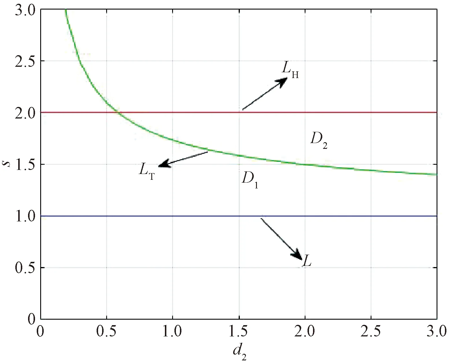
where 0 The Jacobian matrix of Eq.(2) corresponding to the positive equilibriumE*is given by (4) We perturb Eq.(3) around the homogeneous steady stateE*as whereλis the growth rate of perturbation at timet,k(k2=k·k)is the wave number,kis the vector in two dimensions,r=(x,y) is the spatial vector in two dimensions, i(i2=-1) is the imaginary unit andc.c.represents the complex conjugate. Then we have the expression of eigenvalueλ λ2-Tkλ+Dk=0, (5) where Tk=-(d1+d2)k2+T0,Dk=d1d2k4-(a10d2+b01d1)k2+D0, withT0=a10+b01andD0=a10b01-a01b10. From Eq.(4), we haveT0=Q(1-Q)(s-1)-RandD0=RQ(1-Q).Due to 0 LetT0=0, we obtain (6) By calculation, we know that Thus, Hopf bifurcation of Eq.(2) occurs ats=sH. When the self-diffusion termd1>0 andd2>0 under the condition(C1), from the expression ofTk, we know thatTk<0 for anyk>0. Thus, we just need to analyzeDk. Ifa10≤0, then for anyk>0, we haveDk>0. And the positive equilibriumE*of Eq.(3) is stable. Calculation implies that the conditiona10≤0 is equivalent to the following condition(C2) Obviously, if condition(C2) satisfies, then the condition(C1) satisfies. Ifa10>0, there exists someksuch thatDk<0. Thus the positive equilibriumE*of Eq.(3) is unstable. The condition ofa10>0 is equivalent to the following condition(C3) From the expression ofDk, we know that the instability is caused by self-diffusion coefficientd2. This shows that the appearance of the self-diffusion will change the stability of the positive equilibriumE*of Eq.(3). Next, we continue to deduce the conditions of Turing bifurcation. The Turing bifurcation occurs when Re(λk)=0,Im(λk)=0 atk=kT≠0. From the expression ofDk, the critical wave numberkTsatisfies The necessary conditions of Turing instability are given as (7) Simplifying the above Eq.(7), we have the following conditions(C4) and(C5) (8) Summarizing the above analysis, we have the following conclusion. Theorem1Suppose that the parametersRandsare positive, and 0 (i) If the condition(C1) is satisfied, then the positive equilibriumE*of Eq.(2) is locally asymptotically stable fors (ii)We also assume thatd1andd2are positive. (a) If the condition(C2) is satisfied, then the positive equilibriumE*of Eq.(3) is stable. Theorem2Suppose that the parametersR,s,d1andd2are positive, and 0 ProofAccording to the above analysis, if the condition(C5) holds, then the condition(C4) also holds. These two conditions are the result of the simplification of the above Eq.(7) which is the necessary condition of Turing instability. Fig. 1 Bifurcation diagram of Eq.(3) with d1=0.1, Q=0.4 and R=0.24 In this section, we will use the multiple scale method to derive the amplitude equations. Firstly, we choosed2as the control parameter. For the sake of perturbation, we expand the control parameterd2,u,vand the nonlinear term with a small parameterε. Then by bringing them into the equations and comparing the coefficients ofε,ε2andε3, we can get three new equations. Lastly, by using Fredholm solvability conditions, we obtain the amplitude equations. Let and we rewrite Eq.(3) atE*as (9) where Herea10,a01,b10andb01are given by Eq.(4). The others are as follows. We know that the bifurcation parameterd2, the variableu,vandtcan be expressed as[12] (10) (11) t=T0+εT1+ε2T2+o(ε2), (12) which leads to (13) and (14) In addition, the derivative with respect to time is given by whereT1=εt, andT2=ε2t. Then substituting Eqs.(10)-(14) into Eq.(9), we obtain the following linear equations by comparing the coefficients ofε,ε2andε3. (15) (16) (17) The solution to the linear Eq.(15) is (18) (19) Then, the amplitude equations satisfy (20) whereh1=a20p2+2a11p+a02, andh2=b20p2+2b11p+b02. Then the solution to Eq.(16) is given as follows. (21) The coefficients in Eq.(21) are given by solving the sets of linear equations of e0, eikj·r, e2ikj·r, ei(kj-km)·r,j,m=1, 2, 3, then where Taking Eqs.(18) -(21) into Eq.(17), similarly, we have (22) where -m=[(a20+qb20)p+(a11+qb11)](x1+x2)+[(a11+ (a03+qb03)], -n=[(a20+qb20)p+(a11+qb11)](x1+x3)+[(a11+ qb11)p+(a02+qb02)](y1+y3)+(a30+qb30)p3+3(a21+qb21)p2+3(a12+qb12)p+(a03+qb03). (23) Multiplying Eq.(20) and Eq.(22) byε,ε2and merging the variables, we obtain the following amplitude equations. (24) Each amplitude in Eq.(24) can be decomposed into a modeρj=|Aj| and a phase angleφj,j=1, 2, 3. Then substitutingAj=ρjeiφjinto Eq.(24) and separating the real and imaginary parts, we can obtain four differential equations of the real variables as follows. (25) whereφ=φ1+φ2+φ3. The dynamical Eq.(25) possesses five kinds of solutions[12]. (1) The stationary state given by ρ1=ρ2=ρ3=0, is stable forμ<μ2=0 and unstable forμ>μ2. (2) Stripe patterns given by (3) Hexagon patterns are given by (4) The mixed states are given by Takingd2=1.5, then we getμ= -0.052 7, which is in interval(μ1,μ2). We find that the pattern is spot pattern by numerical simulations( shown in Fig. 2). It is consistent with the theoretical results. This paper concentrates on the dynamical behavior of a diffusive predator-prey model with Gompertz growth, which is further rich in biological significance. The necessary conditions for Turing pattern caused by spatial diffusion are given. Then, amplitude equations are derived by multiple scale analysis. In addition, an example by numerical simulations is given. Example 1 shows that spot pattern appears when the control parameter is in the Turing space. This is consistent with our previous theoretical results. The research shows that spatial diffusion plays an important role in the formation of the pattern.


2 Amplitude Equations


3 Conclusions
 Journal of Donghua University(English Edition)2021年5期
