Application of Snell's law in reflection raytracing using the multistage fast marching method

Xingzhong Li ,Wei Zhang

Keywords:reflection raytracing Snell's law traveltime reflection angle

ABSTRAC T Accurate calculations of travel times and raypaths of reflection waves are important for reflection travel time tomography.The multistage shortest path method (MSPM) and multistage fast marching method (MFMM) have been widely used in reflection wave raytracing,and both of them are characterized by high efficiency and accuracy.However,the MSPM does not strictly follow Snell's law at the interface because it treats the interface point as a sub-source,resulting in a decrease in accuracy.The MFMM achieves high accuracy by solving the Eikonal equation in local triangular mesh.However,the implementation process is complex.Here we propose a new method which uses linear interpolation to compute the incident travel time of interface points and then using Snell's law to compute the reflection travel time of grid points just above the interface.Our new method is much simpler than the MFMM;furthermore,numerical simulations show that the accuracy of the MFMM and our new method are basically the same,thus the reflection tomography algorithms which use our new method are easier to implement without decreasing accuracy.Besides,our new method can be extended easily to other grid-based raytracing methods.

1.Introduction

Ray tracing is a classic problem in seismology (Shearer,2019).The purpose of ray tracing is to compute the travel time and raypath of a seismic wave between a source and receiver within a layered or heterogeneous medium.Traditional solutions for this problem include shooting and bending methods.The shooting method (Julian and Gubbins,1977;Bulant,1996) regards the ray equation as an initial value problem,and the ray tracing process continuously adjusts the angle of the ray emitted from the source until it reaches the receiver.The bending method (Julian and Gubbins,1977;Um and Thurber,1987) formulates the ray equation as a boundary value problem by iteratively adjusting the geometry of an initial arbitrary path that joins the source and receiver until it satisfies Fermat's principle.However,both the shooting method and bending method may fail to converge when there are even small velocity variations,and the robustness decreases with the complexity of the medium (Rawlinson and Sambridge,2004a).Low efficiency is another drawback of these two methods because these processes involve a single loop from the source to the receiver.The final difficulty is the selection of the raypath;due to the potential existence of multiple two-point raypaths,neither the shooting method nor the bending method can ascertain which raypath has been selected (Rawlinson and Sambridge,2004a).

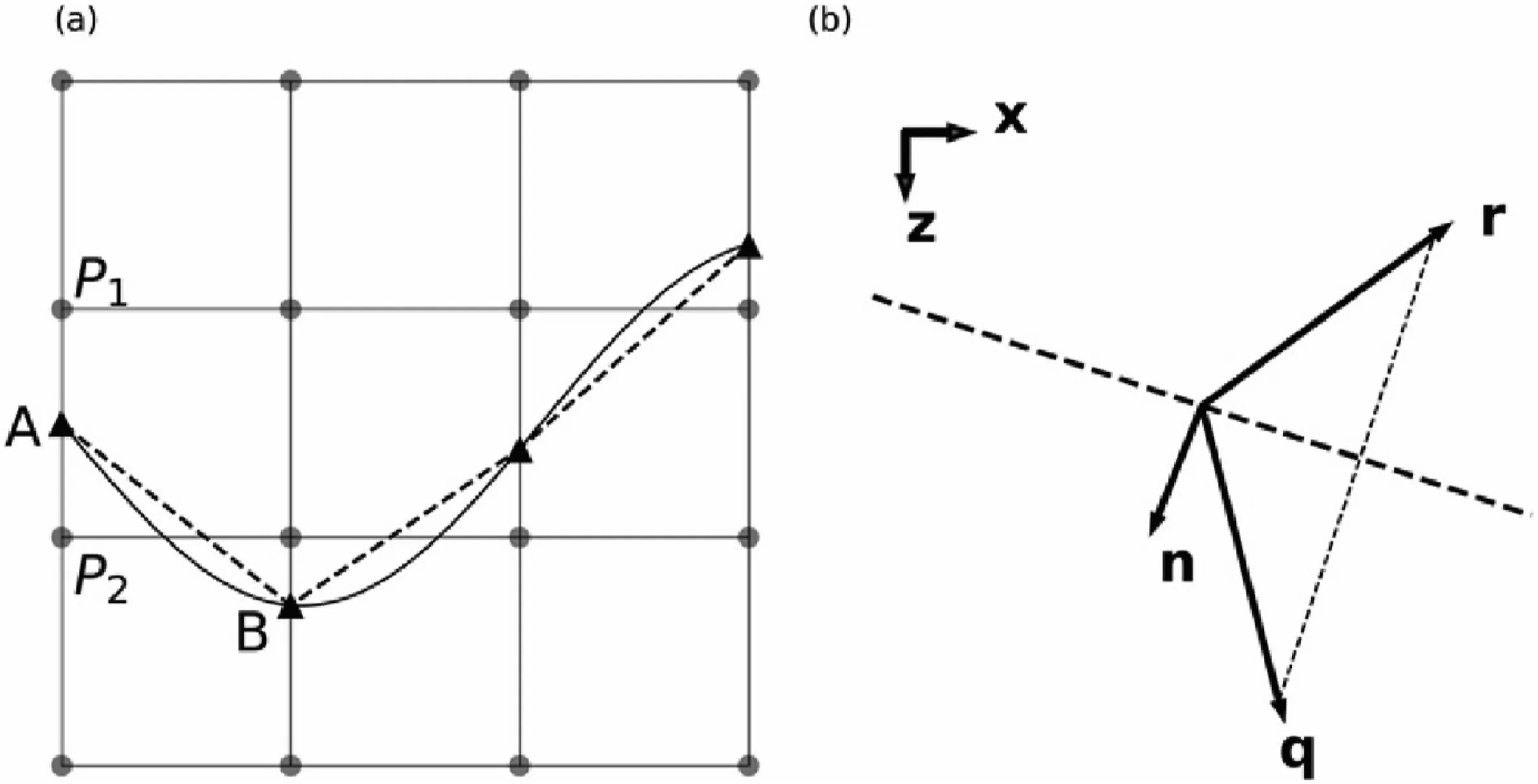
Fig.1.MFMM-Snell in the 2D case.(a) The gray circles denote the grid points and the interface points(black triangles) are located at the vertical grid lines.The solid black curve denotes the true undulating interface,and the dashed lines represent the interface formed by the discretized interface points；(b) The plane where the reflection occurs.The dashed line represents the local reflector,such as AB.n denotes the unit normal of the local reflector,while q and r denote the incident and reflection travel time gradient of the local reflector respectively.

Since the shooting and bending methods suffer from inadequate robustness,poor efficiency,and difficulty in the ray selection process,at present,two main types of grid-based numerical schemes are usually employed to perform ray tracing:finite-difference solution to the Eikonal equation and the shortest path method.Vidale (1988,1990) propose a finite-difference scheme to solve the Eikonal equation by tracking an expanding square or cube throughout a gridded velocity field rather than integrating the travel time along the raypath.The raypath can then be computed with the backward travel time gradient obtained from the travel time calculation.Since this method would fail to obtain head waves travelling along interfaces with large velocity gradients,some modifications to the operators and algorithms have been proposed to overcome the instability related to head waves (Hole and Zelt,1995;Afnimar and Koketsu,2000).Qin et al.(1992) propose an expanding wavefront scheme instead of using expanding squares or cubes to calculate the travel time field.Subsequently,the fast marching method(FMM)(Sethian,1996,1999;Sethian and Popovici,1999;Popovici and Sethian,2002)was proposed.The main difference between the method proposed by Qin et al.(1992) and the FMM is that the FMM uses an entropy-satisfying upwind difference scheme to ascertain the causality of wavefront evolution.In addition,a heap sort algorithm is applied in the FMM to accelerate the process of wavefront evolving by decreasing the computing complexity from O(N^2) to O(NlogN),where N is the total number of grid points in the computational domain.Another technique for solving the problem of box expansion(Vidale,1988,1990)is the fast sweeping method(FSM)(Zhao,2005;Han et al.,2017).The FSM solves the static Hamilton-Jacobi equations using Gauss-Seidel iterations with alternate sweeping orderings,which can cover all possible ray directions without tracking the minimal travel time point along the wavefront.The shortest path method (SPM) (Nakanishi and Yamaguchi,1986;Moser,1991;Zhang and Toksoz,1998;Bai et al.,2007) is another popular grid-based method for raytracing.Instead of solving the Eikonal equation,a network or graph is formed by connecting adjacent velocity points,and then a Dijkstra-like algorithm is applied to find the raypaths with the minimum traveltimes between the source and receivers within the network.Compared with the shooting and bending methods,the grid-based method is more efficient in case of large numbers of sources and/or receivers because the travel time field needs to be calculated only once for each source (Rawlinson and Sambridge,2004a,2005).In addition,the grid-based methods can always provide the right solution even in a complicated velocity structure.Thus,they are more robust than the shooting and bending methods.Finally,the problem of ray selection can be overcame as the obtained traveltime is always the first-arrival travel time.

Hybrid schemes combining grid-based methods with the bending method have become increasingly popular in recent years.Melendez et al.(2015) use the solution of the SPM as an initial estimate for the bending method.This strategy can achieve a good balance between accuracy and efficiency.

While grid-based approaches can be fast and robust and have no difficulty in the ray selection,they usually give only the solution of the first-arrival travel time in a continuous medium,and the reflection travel time field generated at velocity discontinuities cannot be directly obtained.While reflection information is more important than the firstarrival traveltimes for reflection traveltime tomography,several studies have shown how to compute the reflection traveltime using grid-based algorithms.Podvin and Lecomte (1991) and Riahi and Juhlin (1994)track the first-arrival travel times from both the source and the receiver to the entire reflection interface and then apply the Fermat's principle of stationary time to locate the reflection points along the interface.Although this approach can find the reflection travel time and raypath between the source and receiver,the obvious drawback is the poor efficiency because the traveltime field needs to be calculated for each source and receiver.To improve efficiency,Hole and Zelt(1995)suggest the application of Snell's law on calculating the reflection travel time of the grid points just above the reflector.Then,these points are used as secondary sources to propagate the reflection ray to receivers,thus the travel time field only needs to be calculated twice for each shot point.However,this approach only considers the variation of velocity and depth along the vertical direction when it comes to the reflector,thus decreasing the accuracy.

To overcome this problem,Rawlinson and Sambridge(2004a,2004b,2005) and Kool et al.(2006) develop the multistage fast marching method (MFMM),which achieves high accuracy by using irregular triangular (2D) or tetrahedral (3D) mesh near the interface and then solves the Eikonal equation in the irregular grid.But the MFMM is too difficult to implement,especially in 3D case.The use of the multistage strategy for reflection raytracing is also extended to the modified shortest path method (MSPM) by Bai et al.(2009).However,this method treats each point on the reflection interface as a secondary source.As a result,the reflection point could only be at the discrete nodes at the reflector,and the propagation of seismic rays near the reflector does not strictly follow Snell's law.

Zhang et al.(2004)introduce a dynamic network concept to compute the first arrival traveltime in the context of shortest path ray tracing.In every cell,the travel time is computed at particular node by linear interpolation of travel times from adjacent grid points,and then the Fermat's principle of minimum travel time is used to determine the minimum travel time.We adapt this idea to reflection raytracing in the MFMM to allow the reflection point at any position along the reflector using Snell's law,and the incident travel time and gradient of the reflector are computed by linear interpolation rather than solving the Eikonal equation in the irregular grid.In this way,the method is much simpler than the MFMM without decreasing the accuracy,both in 2D and 3D cases.We name this novel method MFMM-Snell.In the following sections,we introduce the new method and then use numerical examples to verify the effectiveness in the reflection raytracing performance with the proposed method,followed by the conclusion.

2.Method

Our new method consists of the following steps:First,the incident travel time and gradient of interface point is computed by linear interpolation.Next,the reflection travel times of the grid points just above the interface are computed by Snell's law.The reflection travel times of the remaining grid points above the reflector are calculated according to the grid points with known reflection travel times by reusing the FMM.

2.1.Incident travel time calculation by linear interpolation

As illustrated in Fig.1a,a reflector can be discretized by a series of equally spaced points that are located at the vertical grid lines,but their depths can be any value,not constrained at the grid points.Since the arrivals that turn at or below the reflector may come earlier than direct waves when the velocities below the reflector are much greater than the velocities above,but do not represent the reflected waves,the velocities of the points below the reflector take the values of the points just above the reflector.For example,the velocities of the grid pointP2and below take the velocity of the grid pointP1,similar to the vertical lines.Then,the FMM is used to calculate the incident travel times throughout the model.Thus,the incident travel times and gradients of interface points can be obtained by linear interpolation:

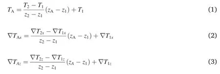
whereTAand（∇TAx，∇TAz）are the incident travel time and its gradient of the interface point A（xA，zA）,Tiand（∇Tix，∇Tiz）are the incident travel time and its gradient of the grid pointPi（xi，zi）.

2.2.Reflection travel time calculation based on Snell's law

After the incident travel time and its gradient are obtained at all interface points,Snell's law can be used to calculate the reflection travel times of the grid points just above the reflector.As illustrated in Fig.1a,point A and B are two adjacent interface points,and pointP1is a grid point just above the reflector.The traveltimes and gradients at A and B are already fixed and can be expressed asTAandTBand as ∇TA=（∇TAx，∇TAz）and ∇TB=（∇TBx，∇TBz）,respectively.The reflection travel time and gradient ofP1is about to calculate and can be expressed asT1and ∇T1=（∇T1x，∇T1z）.

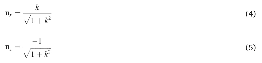
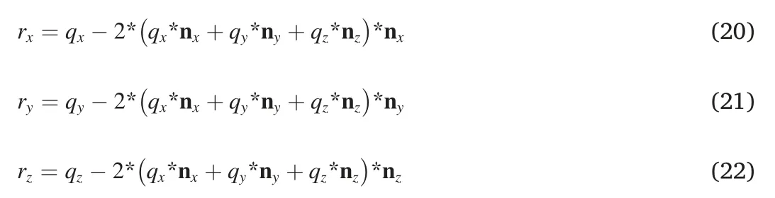
As illustrated in Fig.1b,n（nx，nz）represents the unit normal of the local reflector AB and can be expressed as:

wherekis the slope of line AB and can be expressed as:

and the equation of line AB can be expressed as:

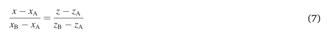
Fig.2.MFMM-Snell in the 3D case.The black solid lines represent the regular velocity grid.P1,P2,P3,and P4 (black dots)are four adjacent interface point and the dashed black line represents the plane that fitted by the four adjacent interface point.

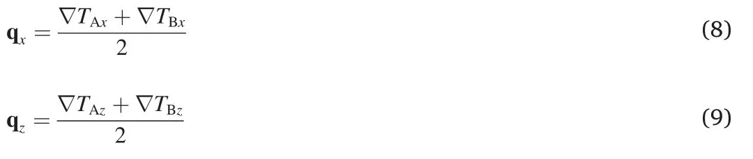
We assume the wavefront is local planar and take the average of the incident travel time gradient of point A and B as the incident travel time gradient q（qx，qz）of the local reflector AB:

According to Snell's law,Equa.(10)is obtained below:

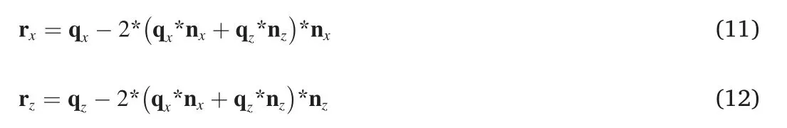
where r（rx，rz）is the reflection travel time gradient of the local reflector AB,which can be derived from Equa.(10):

Then the equation of the ray which arrives at grid pointP1after reflection can be expressed as:

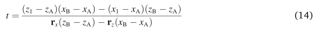
Combine Equas.(7)and(13),we obtain Equa.(14):

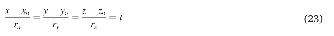
Then the reflection point C（xC，zC）can be obtained by combining Equas.(13)and(14):

Because reflection point C lies on AB,the solution should satisfy:

Then,we can obtain the travel time ofP1by:

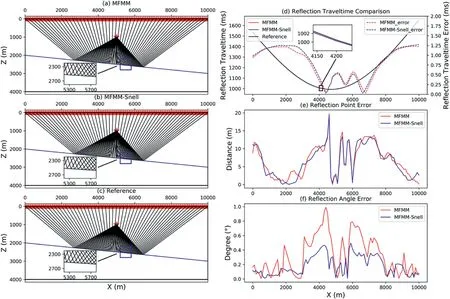
Fig.3.Homogeneous model with a dipping interface in the 2D case.(a),(b) and (c) are Raypaths of the MFMM,MFMM-Snell,and the reference solution,respectively.The red star represents the source and red triangles represent receivers.The blue straight line represents the dipping interface and the blue box shows a magnified view of the raypaths;(d) reflection travel time comparison among the MFMM,MFMM-Snell,and the reference solution,where the solid lines represent the reflection travel time (left axis) and the dashed lines represent the travel time error(right axis);(e) reflection point error of the MFMM and MFMM-Snell;(f)reflection angle error of the MFMM and MFMM-Snell.

whereTCis the incident travel time of reflection point C and can be obtained by linear interpolation usingTAandTB.｜P1C｜represents the distance between reflection point C and grid pointP1,and S is the average slowness of reflection point C and grid pointP1.T1needs to be computed using each two adjacent interface points around pointP1by Snell's law,and the minimum value is always selected;that is,the value we compute is the first-arrival reflection travel time.

After the reflection travel times of all grid points just above the reflector are fixed,the reflection travel times of the remaining grid points can be obtained by reusing the FMM,and then the reflection raypath can be tracked according to the travel time gradients.

2.3.MFMM-Snell in 3D case

MFMM-Snell can be extended to the 3D case easily.As shown in Fig.2,pointO（xO，yO，zO）is the grid point just above the reflector whose reflection travel timeTOis about to calculate,P1toP4are four adjacent interface points that are located on each vertical grid line.The depth of the four points are not constrained at the grid points and could be any value.The incident travel time and gradient of these interface points can be obtained by linear interpolation such as the 2D case.Due to the fact that these four points may not be exactly in the same plane,we use an approximate plane to fit them.The average of the unit normal of the planeP1P2P3,P2P3P4,P3P4P1andP4P1P2are taken as the unit normal of the fitted plane which can be expressed as n=（nx，ny，nz）.In addition,the midpoint M（xm，ym，zm）of the four points is assumed on the fitted plane,thus the fitted plane can be determined by the point normal form:

The incidence and reflection travel time gradient are denoted asq=（qx，qy，qz）andr=（rx，ry，rz）respectively,and Snell's law can be expressed with Equa.(10),thus:

Then the equation of the ray which arrives at grid point O after reflection can be expressed as:

Combining Equa.(19)and(23),we obtain the solution of parametert.As a result,the position of reflection point can be calculated using Equa.(23).The reflection travel time of point O can be computed through the same approach used in the 2D case.

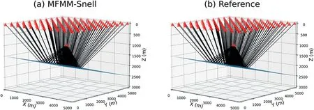
Fig.4.Homogeneous model with a dipping interface in the 3D case.The red star represents the source and red triangles represent receivers.The blue surface represents the dipping interface.(a) Raypaths of MFMM-Snell;(b) Raypaths of the reference solution.

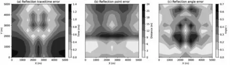
Fig.5.Errors of the homogeneous model with a dipping interface in the 3D case.(a)Reflection travel time error of MFMM-Snell;(b)Reflection point error of MFMMSnell;(c) Reflection angle error of MFMM-Snell.

Fig.6.Homogeneous model with an undulating interface in the 2D case.(a),(b) and (c) Raypaths of the MFMM,MFMM-Snell,and the reference solution,respectively.The red star represents the source and red triangles represent receivers.The blue curve represents the undulating interface and the blue box shows a magnified view of the raypaths;(d)reflection travel time comparison among the MFMM,MFMM-Snell,and the reference solution,where the solid lines represent the reflection traveltime(left axis)and the dashed lines represent the travel time error(right axis);(e)reflection point error of the MFMM and MFMM-Snell;(f)reflection angle error of the MFMM and MFMM-Snell.

3.Numerical examples

3.1.Homogeneous model with a dipping interface

First,we test our method using a dipping reflector that lies within a homogeneous velocity field in the 2D case.The grid spacing of the MFMM (Rawlinson and Sambridge,2004a,2004b,2005,2004b) and MFMM-Snell(our method)are both 50 m.For this example,the reference solution is calculated by using a very fine spacing (0.01 m) along the interface and choosing the interface point with the minimum error between the incident angle and the reflection angle as the real reflection point.The results of the MFMM,MFMM-Snell,and the reference solution are illustrated in Fig.3.Rays obtained by the MFMM (Fig.3a) and MFMM-Snell(Fig.3b)are both straight and evenly distributed along the interface,which are almost perfectly matched with the reference solution(Fig.3c).

The reflection travel times (Fig.3d) of the MFMM and MFMM-Snell do not exhibit notable discrepancies with regard to the reference solution.The magnitude of the reflection travel time error (Fig.3d) of both the MFMM and MFMM-Snell are less than 1.25 ms,which is quite small compared with the reflection travel time (larger than 1000 ms),indicating that both the MFMM and MFMM-Snell can achieve accurate reflection travel time computation.The discrepancy in the reflection point error(Fig.3e)is very small.The maximum reflection point error of both the MFMM and MFMM-Snell are less than 20 m,which is relatively small compared with the scale of the model(10 000 m＊4000 m)and the grid spacing (50 m).The reflection angle error (Fig.3f) from MFMMSnell is smaller than that of the MFMM for some receivers,but the discrepancy is very small (The maximum errors of MFMM-Snell and MFMM are 0.5°and 1°receptively).In other words,both the MFMM and MFMM-Snell can obtain accurate reflection angles.The results of this example demonstrate that MFMM-Snell can achieve the same precision as the MFMM for simple models with simple reflectors in the 2D case.

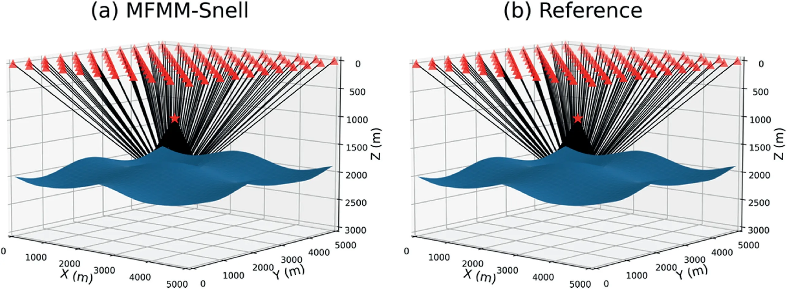
Fig.7.Homogeneous model with an undulating interface in the 3D case.The red star represents the source and red triangles represent receivers.The blue surface represents the undulating interface.(a) Raypaths of MFMM-Snell;(b) Raypaths of the reference solution.

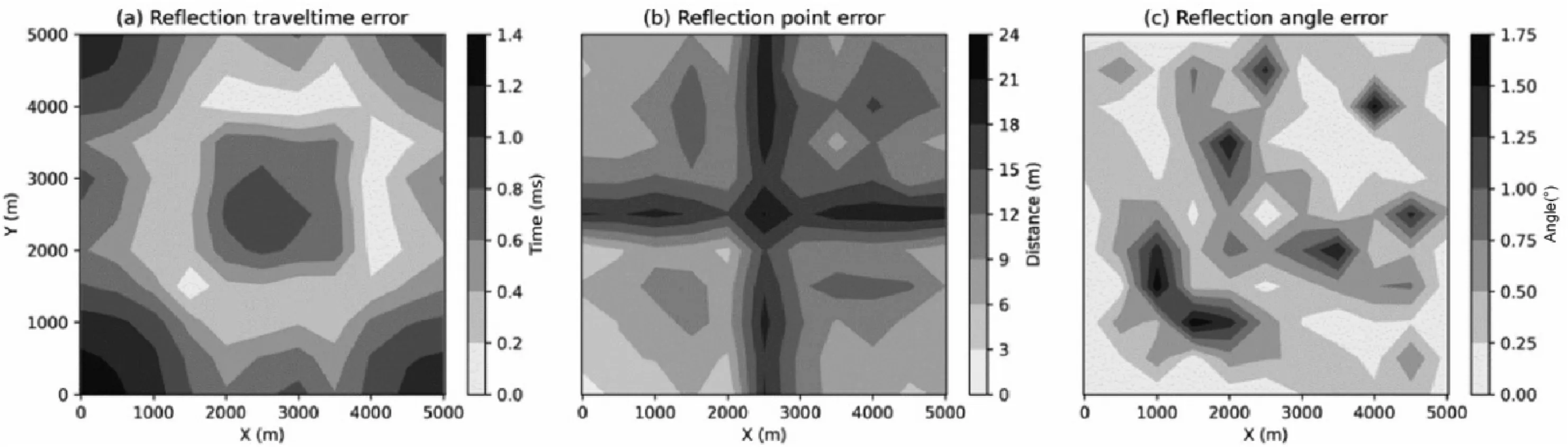
Fig.8.Errors of the homogeneous model with an undulating interface in the 3D case.(a) Reflection travel time error of MFMM-Snell;(b) Reflection point error of MFMM-Snell;(c) Reflection angle error of MFMM-Snell.

Fig.9.The Marmousi model with a sharp-edge interface in the 2D case.(a),(b)and(c)Raypaths of the MFMM,MFMM-Snell,and the reference solution,respectively.The red star represents the source and red triangles represent receivers.The blue curve represents the sharp-edge interface;(d) reflection travel time comparison among the MFMM,MFMM-Snell,and the reference solution,where the solid lines represent the reflection travel time (left axis) and the dashed lines represent the travel time error (right axis);(e) reflection point error of the MFMM and MFMM-Snell;(f) reflection angle error of the MFMM and MFMM-Snell.

Fig.10.The Marmousi model with a sharp-edge interface in the 3D case.The red star represents the source and red triangles represent receivers.The blue surface represents the sharp-edge interface.(a) Raypaths of MFMM-Snell;(b) Raypaths of the reference solution.

Then we test MFMM-Snell using a homogeneous model with a dipping interface in the 3D case,in which the grid spacing of MFMMSnell is 50 m.Because the MFMM is too complex to implement in the 3D case,we only compare the results of MFMM-Snell and the reference solution which can be obtained in the same way in the 2D case previously.As illustrated in Fig.4,the raypaths obtained by MFMM-Snell(Fig.4a) are almost perfectly matched with the reference solution(Fig.4b).Fig.5 shows the reflection travel time error (Fig.5a),the reflection point error (Fig.5b),and the reflection angle error (Fig.5c),respectively.The maximum value of the reflection travel time error,the reflection point error and the reflection angle error are about 1.4 ms,24 m,and 0.7°respectively,which are relatively small and close to the maximum reflection travel time error in the 2D case with the same grid spacing.The results of this example prove that MFMM-Snell can achieve the same precision as 2D in the 3D case for simple model with simple reflector.

3.2.Homogeneous model with an undulating interface

The second example is slightly more complex than the first.This example involves an undulating interface that lies within a homogeneous medium,and the grid spacing of the MFMM and MFMM-Snell are both 50 m.The reference solution can be obtained in the same way as that for example 1 since the velocity field is homogeneous.Fig.6a,6b,and 6c illustrate the raypaths of the MFMM,MFMM-Snell,and the reference solution,respectively.Similar to example 1,the rays computed by both the MFMM and MFMM-Snell are straight and evenly distributed along the interface,which are quite close to the reference solution.Fig.6d,6e,and 6f show comparisons between the MFMM and MFMM-Snell for the reflection travel time error,reflection point error,and reflection angle error,respectively.Similar to the first example,it is clear that both the MFMM and MFMM-Snell can achieve high accuracy.Meanwhile,the discrepancy between the results of the two methods is quite small.The maximum value of the reflection travel time error,the reflection point error and the reflection angle error are approximately 1.5 ms and 1.4 ms,15 m and 14 m,and 2.1°and 1.7°for MFMM and MFMM-Snell respectively.The results of this example prove that MFMM-Snell can achieve the same precision as MFMM for simple models with undulating interfaces.

Then we test MFMM-Snell using a homogeneous model with an undulating interface in the 3D case,and the grid spacing of MFMM-Snell is 50 m.Similar to the first example,we compare the results of MFMM-Snell and the reference solution.As illustrated in Fig.7,the raypaths obtained by MFMM-Snell (Fig.7a) are extremely close to the reference solution(Fig.7b).Fig.8 shows the reflection travel time error (Fig.8a),the reflection point error (Fig.8b),and the reflection angle error (Fig.8c),respectively.The maximum value of the reflection travel time error,the reflection point error,and the reflection angle error are about 1.4 ms,24 m and 1.75°respectively,which are quite small and close to the maximum reflection travel time error in the 2D case under the same grid spacing.The results of this example prove that MFMM-Snell can achieve the same precision as 2D in the 3D case for simple model with undulating reflector.

3.3.Marmousi model with an undulating interface

The third example in this paper is more complicated than the previous two.In this scenario,a sharp edge interface lies within the Marmousi model(Versteeg,1994).The grid spacing of the MFMM and MFMM-Snell are both 50 m and all the raypaths are calculated in the smoothed Marmousi model.Since the velocity field is complex,we cannot obtain the reference solution for the reflected wave in the same way as that used in examples 1 and 2.However,we can obtain a highly accurate result to approximate the reference solution by using a small grid spacing(1 m).Fig.9a,9b,and 9c illustrate the raypaths of the MFMM,MFMM-Snell,and the reference solution,respectively.It is obvious that the rays obtained by the MFMM and MFMM-Snell both are close to those of the reference solution.Similar to the previous two examples,the reflection travel time error (Fig.5d),the reflection point error (Fig.5e) and the reflection angle error(Fig.5f)also show a slight difference between the MFMM and MFMM-Snell,and all of them are relatively small compared with the model scale (9192 m ＊ 2904 m) and grid spacing (50 m).The results of this example demonstrate that MFMM-Snell can basically achieve the same accuracy as MFMM for complex models with sharp-edge interfaces.

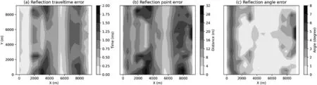
Fig.11.Errors of the Marmousi model with a sharp-edge interface in the 3D case.(a)Reflection travel time error of MFMM-Snell;(b)Reflection point error of MFMMSnell;(c) Reflection angle error of MFMM-Snell.

Next we test MFMM-Snell using a Marmousi model with a sharp-edge interface in the 3D case,which is expanded from the 2-D Marmousi model along they-direction,and the grid spacing of MFMM-Snell is 50 m.Similar to the previous two examples,we compare the results of MFMMSnell and the reference solution which can be obtained in the same way used in the 2-D case previously.As illustrated in Fig.10,the raypaths obtained by MFMM-Snell(Fig.10a)are extremely close to the reference solution (Fig.10b).Fig.11 shows the reflection travel time error(Fig.11a),the reflection point error (Fig.11b),and the reflection angle error(Fig.11c),respectively.The maximum value of the reflection travel time error,the reflection point error,and the reflection angle error are about 2 ms,32 m,and 8°respectively,which are quite small and close to the maximum reflection travel time error in the 2-D case with the same grid spacing.The results of this example prove that MFMM-Snell can achieve the same precision as 2-D in the 3-D case for complex model with sharp-edge reflector.

4.Conclusion

Accurate calculations of the travel time and raypath of reflection waves are important for reflection travel time tomography.The multistage shortest path method(MSPM)calculates the downgoing rays to the reflectors and uses arrival time at the reflectors as secondary sources to calculate the upgoing rays to the receivers.In this procedure,the upgoing rays may not strictly satisfy Snell's law,thus decreasing the accuracy.The multistage fast marching method (MFMM) achieves high accuracy by solving the Eikonal equation in the local triangular (2D.However,the implementation process is complex especially in the 3D case.In this study,we develop an MFMM-Snell method to simplify the complexity of the MFMM without reducing accuracy.MFMM-Snell uses linear interpolation to calculate the incident travel time and gradient of the reflector,and then computes the reflection travel times of points just above the reflector based on Snell's law.The reflection travel times of the remaining points above the reflector are calculated according to the points with known reflection travel times obtained by the FMM.We note that the FMM in MFMM-Snell method can be replaced by other grid-based raytracing methods,such as SPM and FSM.Hence,our new method can be extended easily to other grid-based raytracing methods.The proposed MFMM-Snell method is verified using both simple and complex velocity models.The results indicate that our proposed MFMM-Snell method can achieve the same accuracy as the MFMM.

Acknowledgements

This research is jointly sponsored by National Natural Science Foundation of China(Grant No.U1901602),Shenzhen Key Laboratory of Deep Offshore Oil and Gas Exploration Technology (Grant No.ZDSYS20190902093007855),Shenzhen Science and Technology Program (KQTD20170810111725321).This study is also sponsored by the China Earthquake Science Experiment Project of China Earthquake Administration (Grant No.2018CSES0101).