Viscoelastic relaxation of the upper mantle and afterslip following the 2014 MW 8.1 Iquique earthquake

Zhiping Hu,Yan Hu ,Segun Steven Bodunde

Mengcheng National Geophysical Observatory,School of Earth and Space Sciences,University of Science and Technology of China,Hefei,230000,China

Keywords:2014 MW 8.1 Iquique earthquake Postseismic viscoelastic relaxation Afterslip Finite element model Lithosphere geodynamics Upper mantle rheology

ABSTRAC T An improved understanding of postseismic crustal deformation following large subduction earthquakes may help to better understand the rheological properties of upper mantle and the slip behavior of subduction interface.Here we construct a three-dimensional viscoelastic finite element model to study the postseismic deformation of the 2014 MW8.1 Iquique,Chile earthquake.Elastic units in the model include the subducting slab,continental and oceanic lithospheres.Rheological units include the mantle wedge,the oceanic asthenosphere and upper mantle.We use a 2 km thick weak shear zone attached to the subduction fault to simulate the time-dependent stressdriven afterslip.The viscoelastic relaxation in the rheological units is represented by the Burgers rheology.We carry out grid-searches on the shear zone viscosity,thickness and viscosity of the asthenosphere,and they are determined to be 1017 Pa s,110 km and 2×1018 Pa s,respectively.The stress-driven afterlsip within the first two years is up to～47 cm and becomes negligible after two years(no more than 5 cm/yr).Our results suggest that a thin,low-viscosity oceanic asthenosphere together with a weak shear zone attached to the fault are required to better reproduce the observed postseismic deformation.

1.Introduction

Research on the postseismic crustal deformation following large subduction earthquakes can help us better understand deformation processes in the convergent margins.Wang et al.(2012) proposed that the interplay of three primary processes controls the postseismic crustal deformation after a great subduction earthquake.These include a seismic afterslip occurring mostly around the coseismic rupture zone,viscoelastic relaxation in the upper mantle and relocking of the subduction fault.Hu and Wang,2012 reported that a thin,low-viscosity asthenospheric layer beneath the elastic oceanic lithosphere is required to better reproduce the observed postseismic uplift following the 2012MW8.6 Indian Ocean earthquake occurring within the Indian oceanic plate.

The northern Chile-southern Peru seismic gap that broke in 1877 is probably the most mature seismic gap along the South American plate boundary (Schurr et al.,2014).Comte et al.(1995) inferred that the downdip limit of the seismogenic zone in this region is approximately at the depth of 60 km.The magnitude 8.1 Iquique earthquake occurred on April 1,2014 following a protracted series of foreshocks (Ruiz et al.,2014;Kato et al.,2016).According to the United States Geological Survey (USGS) the hypocenter was located at 19.642°S,70.817°W with a depth of 23 km.The largest aftershock with Mw7.7 occurred southeast of the main shock epicenter after two days.Coseismic slip models have been proposed by teleseismic inversion (Lay et al.,2014;Yagi et al.,2014),tsunami inversion of offshore DEAR waveform (Lay et al.,2014),GPS data(Shrivastava et al.,2019)and a joint inversion of teleseismic,local strong motion records and GPS data(Schurr et al.,2014).Although these models show significant differences such as the amplitude,extent,location,and updip limit of the primary slip zone,they have similar first-order features.For example,all rupture models do not propagate to the trench (Duputel et al.,2015).The moment magnitude estimated by these published studies are in a range ofMW8.0-8.2 (Gusman et al.,2015).

Hoffmann et al.(2018)inverted the afterslip distribution in an elastic half space at three time periods after removing the effects of the viscoelastic relaxation of the upper mantle assuming the Maxwell viscosity in the continental mantle and oceanic mantle to be 2 × 1019Pa s and 1020Pa s,respectively.Their model showed that cumulative peak afterslip within the first 2 years after the Iquique earthquake was 89.0+1.2/-0.4 cm,mostly at the depth range between 30 and 45 km and surrounding the downdip of the rupture area.After 2 years,the afterslip became much smaller (less than 5 cm/year),and the relocking of the fault became dominant.However,their model may not resolve potential shallow afterslip above 15 km due to limits of available GPS data.Shrivastava et al.(2019) derived two main patches of afterslip within 273 days following the largest aftershock.Accumulated slip of the northern patch was up to 76 cm,whereas the southern patch had a maximal slip of 78 cm.Their result showed that the cumulative postseismic moment released through afterslip during the 273 days was 3.27× 1020N m (～MW7.61),which was accounted for～41.8 % of the moment released via the seismic process.However,the published studies ignored the viscoelastic response of the stress-driven afterslip and rheological heterogeneities in the oceanic upper mantle that together may play an important role in controlling the near-field postseismic deformation.

In this work,we processed four-year postseismic displacements of 19 continuous GPS stations after the Iquique earthquake to study the rheological structure of the northern Chile subduction zone.Based on previous studies on other convergent margins,such as the Northeast Japan(Hu et al.,2016a;Sun et al.,2014),Alaska (Suito and Freymueller,2009),Cascadia and Sumatra subduction zone (Hu and Wang,2012),we constructed a three-dimensional (3-D) viscoelastic finite element model to study the postseismic deformation of the Iquique earthquake.

2.GPS data and model setup

2.1.Postseismic GPS observations

We collected and processed daily time series of 19 continuous GPS stations from the UNR database (http://geodesy.unr.edu).We take the following steps to derive the postseismic displacements from the GPS time series.(1) We extract the GPS time series from 2011 to 2014 before the Iquique earthquake to estimate the long-term secular,annual and semi-annual variations.(2) We correct the time series between April 1st,2014 and April 1st,2018 for the pre-earthquake trends obtained in step(1).(3) We fit the corrected four-year time series after the Iquique Earthquake using logarithmic and exponential functions of time,whereaandbare constants,tis the time,and τlogand τexpare the characteristic time constants of the logarithmic and exponential terms,respectively.τlogand τexpare determined for each GPS station through a grid search method.(4) We then calculate postseismic displacements between any two time epochs from the fitted postseismic curve.For those stations that were discontinued two or more years after the Iquique earthquake,we calculate the 4-year-postseismic displacements through the extended fitted curve.

One year after the 2014 event,stations north of 21°S near the rupture region record maximum cumulative horizontal displacements of up to～11.2 cm in a similar direction to the coseismic motion (for example,station ATGN,red arrow in Fig.1a).The latitudinal displacement gradient around the peak slip area at 20°S is not symmetric.The displacements decrease～8 cm within the first 100 km southward,whereas the decrease amount is～5 cm within the first 100 km northward.Displacements of stations 200 km from peak slip region are less than 1 cm(for example,station URUS,blue arrow in Fig.1a).In the horizontal direction the North component gradient is larger than that of the east component.Displacements of stations 200 km from the coast around 20°S are less than 1 cm.

All the stations within 200 km from the peak slip region underwent subsidence one year after the event.Stations around 20°S recorded cumulative vertical displacements of up to～3 cm.Two of three far-field stations with smaller errors recorded an uplift of～5 mm.

2.2.Stress-driven afterslip

The understanding on the distribution and evolution of the afterslip following subduction zone earthquake has been limited by existing observational capabilities of offshore geodetic networks.A conventional method to study afterslip following an mainshock is to invert the surface geodetic observations in an elastic half space after removing the viscoelastic relaxation effect of the upper mantle.This method ignores the interaction of the time-dependent afterslip and the relaxation of the upper mantle,which may result in an overestimation of afterslip at greater depths.

Following previous studies of postseismic deformation of the 1999MW7.5 Izmit earthquake (Hearn et al.,2002) and 2011MW9.0 Tohoku(Hu et al.,2016a)earthquakes,we apply a low-viscosity shear layer over the fault to simulate the stress-driven afterslip(thin green layer in Fig.2).The afterslip is calculated by differencing the displacements of the bottom and corresponding top surface of the shear zone.There is tradeoff between the thickness and viscosity of the shear zone.Considering the deformation gradient near the fault and the element size required to reduce numerical artifacts,we used the same 2 km thick shear zone as in Hu et al.(2016).For simplicity,we assume that there is no along-strike and lateral variations in the rheological property of the shear zone.The range of the shear zone is between latitudes of 18°S and 22°S,～200 km from the main rupture area.

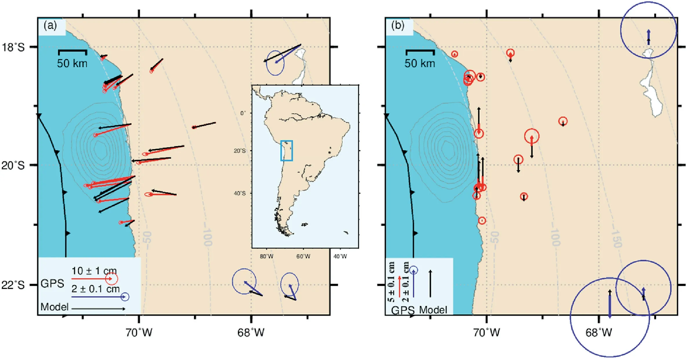
Fig.1.Comparison of GPS observations with model predictions.Red and blue arrows represent GPS observations at different scales in the near-and far-field,respectively.Black arrows represent model predictions.(a) Horizontal cumulative postseismic displacements of within one year after the earthquake.The inset shows the study region in a larger tectonic map of the south America.(b) Vertical cumulative postseismic displacements of within one year after the earthquake.(For interpretation of the references to color in this figure legend,the reader is referred to the Web version of this article.)

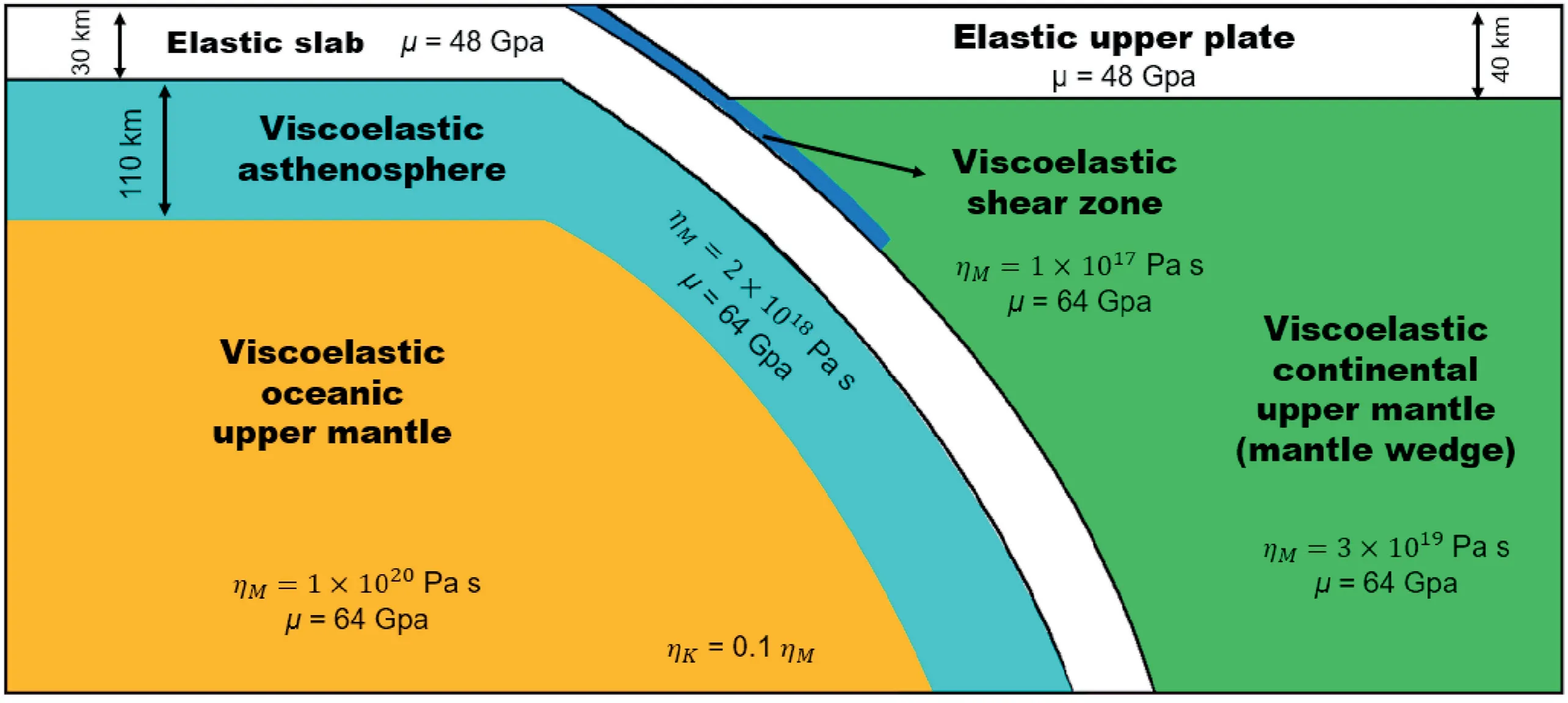
Fig.2.Conceptual representation of the finite-element model.The model includes an elastic slab and elastic upper plate (white color blocks),a viscoelastic mantle wedge(green),an oceanic mantle(blue and brown),and a shear zone attached to the plate interface(navy blue).μ is the shear modulus.The steady-state viscosity values of ηM are 10 times the corresponding transient viscosity ηK.The viscosity values represent the preferred model parameters described in section 3.2.(For interpretation of the references to color in this figure legend,the reader is referred to the Web version of this article.)

2.3.Finite element model

Our 3D viscoelastic finite element model is based on previous studies on other subduction zones,such as,the Chile,Alaska,Cascadia,Northeast and Sumatra subduction zones (e.g.,Wang et al.,2012;Suito and Freymueller,2009;Hu et al.,2016a,2016b).The model includes an elastic upper plate,an elastic subducting slab,a viscoelastic mantle wedge,and a viscoelastic oceanic upper mantle (Fig.2).Based on previous numerical models of the northern Chile subduction zone and seismic studies on the structure in this region and estimates of Contreras-Reyes and Osses(2010),we assume the elastic thickness of the continental and oceanic lithosphere to be 40 km and 30 km,respectively.Unlike previous research on simulating the afterslip,we use a weak shear zone to simulate the time-dependent,stress-driven afterslip(see previous section 2.2).The coseismic slip distribution of the earthquake derived by Schurr et al.(2014)is kinematically prescribed over the fault by adding cohesive cells for the fault surface.

The shear moduli of the elastic lithosphere and viscoelastic upper mantle are assumed to be 48 GPa and 64 GPa(Hu et al.,2004;Li et al.,2015),respectively.The shear modulus of the weak shear zone is assumed to be 6.4 GPa to better simulate the rapid decay of the afterslip(Hu et al.,2016a).The Poisson's ratio and rock density of the whole domain are assumed to be 0.25 and 3.3×103kg/m3,respectively.

We apply the bi-viscous Burgers rheology to represent the viscoelastic relaxation of the upper mantle and the shear zone.In this work,ηKin all the viscoelastic elements is assumed to be one order of magnitude lower than ηM.Following previous studies(Hu et al.,2016a)we assume that the shear modulus in the Maxwell element is the same as that of the Kelvin element.

We manually derive 30 latitude-parallel profiles of the subduction interface based on the SLAB1.0(Hayes et al.,2012)and locations of the arc.We then develop the 3D finite element mesh from the slab profiles using meshing software Trelis (www.csimsoft.com).The element size is on the order of 1 km near the fault and up to 500 km more than 1 000 km from the rupture area.The mesh consists of 51502 nodal points in 284 117 quadratic elements.Our model has a length of 3 000 km along strike and a width of 3500 km perpendicular to the strike extending vertically to 2 000 km.All numerical simulations in our research are solved with the finite element modelling software Pylith(Aagaard et al.,2013).The boundary conditions are assigned to be Dirichlet boundary conditions in Pylith.

3.Model results

We apply a systematic grid-search approach to determine three model parameters,that is,the viscosity of the shear zone(ηS),thickness(DA)and viscosity(ηA)of asthenosphere.We vary DA,ηAand ηSwithin the ranges of 40-160 km,1017-1020Pa s and 1019-1022Pa s,respectively(Fig.3).We start with a coarse grid,and then narrowed down a preferred model with a finer grid.We run 154 test models in total.Then we present the fit of the preferred model to the GPS observations and model predicted distribution and evolution of afterslip.

We evaluate the test models through calculating the weighted χ2misfit:

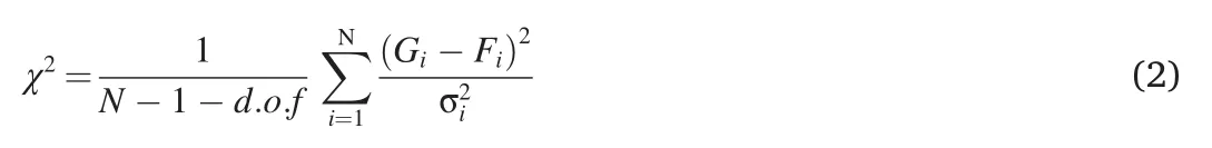
whereGandFrepresent GPS displacement observations and model predictions,respectively,irepresents the station number,the degrees of freedom d.o.f.=3 in this work are for the three free variable model parameters,is the variance of the GPS observation,andNis the total number of GPS stations.

3.1.Lowest misfit model

If we consider χ2only in the horizontal direction,the test model that best fits the horizontal GPS displacements cannot predict the observed subsidence of near-field stations (Fig.3a).If we consider χ2only in the vertical direction,a ηAvalue on the order of 1017Pa s produces a better fit to the vertical component (Fig.3b),but the prediction to horizontal components becomes worse(results not shown).

If we consider χ2in both the horizontal and vertical directions,all three model parameters are constrained within a relatively narrow range(Fig.3c).The preferred lowest misfit model(LMM)with the lowest χ2has ηS=1017Pa s,DA=110 km and ηA=2 × 1018Pa s.The first order rheological properties obtained in this work is consistent with that of previous studies(e.g.,Hu et al.,2016a,2016b;Sun et al.,2018).

The LMM reproduces the first-order pattern of the GPS observations in the horizontal direction (black arrows in Fig.1a).The LMM well predicts up to～10 cm seaward motion of stations 50 km away from rupture area one year after the earthquake.The LMM can overall reproduce the magnitudes of GPS observations for stations near the coseismic rupture area,whereas there are a little off in directions.There is a tendency for stations along the western coast to diverge towards both southern and northern edges of the coseismic rupture area,which may be due to the high-order heterogeneous distribution of afterslip.The LMM does not reproduce the observed subsidence near the coast(black arrows in Fig.1b).The error is larger than processed value in vertical directions for stations more than 50 km from rupture area.The predictions of the LMM on the evolution of displacement within 4 years also matches the general curvature of the observed GPS time series.The curvature fit at three example GPS stations is shown in Fig.4.

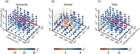
Fig.3.Misfit of 154 test models.Each cube represents one test model.The black-outlined cube represents the model with the lowest χ2 value in each scenario.(a)The χ2 misfit calculated only with horizontal components.(b) The χ2 misfit calculated only with the vertical component.(c) The χ2 misfit calculated with both horizontal and vertical components.

In general,the near-field deformation near the coseismic rupture area is greatly affected by the complicated distribution of afterslip.The fit to GPS observations can be improved by considering other deformation processes,such as poroelastic rebound and relaxation of lower crust beneath the volcanic arc.

3.2.Trade-off among model parameters

To better understand the trade-off between three model parameters,we study the individual contribution of the viscoelastic units to the surface deformation.We carry out four test models based on the preferred lowest misfit model(LMM)obtained in section 3.1(also shown in Fig.5).In each test model,we allow the viscoelastic relaxation only in one rheological unit while the other elements are set to be elastic.

We summarize the effects of individual rheological elements units as follows.For horizontal component,the relaxation of asthenosphere causes landward motion offshore (Fig.6a) while afterslip and the relaxation of mantle wedge control the postseismic seaward motion mainly on land (Fig.6b and 6d).For the vertical components,the relaxation of asthenosphere causes subsidence near rupture zone offshore and uplift farther inland.Afterslip causes uplift updip of the afterslip zone on fault and subsidence downdip.Relaxation of mantle wedge cause uplift close to the trench.Effects of the relaxation in the oceanic upper mantle is negligibly small both in the horizontal and in the vertical directions(Fig.6c).

Fig.4.Comparison of observed 4-yr GPS time series with the predictions of lowest misfit model at three example stations.Red dots with 1σ uncertainties error bars represent the GPS observations.Black lines represent model prediction.Upper,middle and lower panels represent displacements in the East,North,and vertical directions,respectively.(a) Time series recorded at station ATJN.(b) Time series recorded at station PCCL.(c) Time series recorded at station URUS.(For interpretation of the references to color in this figure legend,the reader is referred to the Web version of this article.)

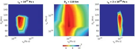
Fig.5.Tradeoff among the viscosity in the shear zone (ηS),the thickness (DA) and the viscosity (ηA) of the oceanic asthenosphere.(a) Trade-off between DA and ηA while ηS is fixed at 1017 Pa s.(b) Trade-off between ηS and ηA while DA is fixed at 110 km.(c) Trade-off between DA and ηS while ηA is fixed at 2 × 1018 Pa s.

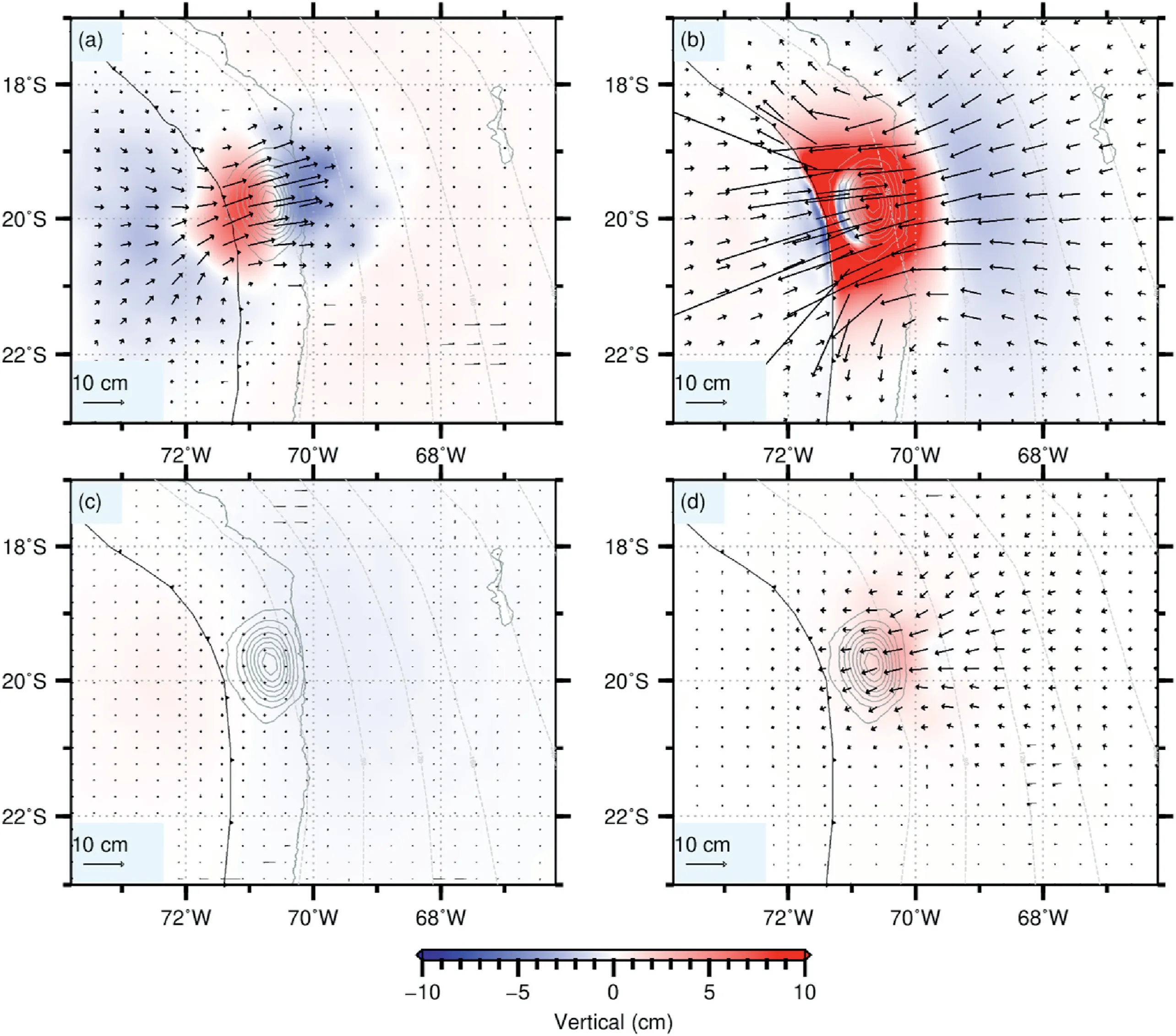
Fig.6.Individual contributions of the relaxation in four rheological units to the surface deformation of model.Viscosities of elements are the same value as that in the lowest misfit model (Fig.3).Black arrows and contours represent cumulative 2 years postseismic displacements in horizontal and vertical components,respectively.Gray contours represent coseismic slip contour of the 2014 Iquique earthquake (Schurr et al.,2014),(a) Viscoelastic relaxation only in the oceanic asthenosphere.(b) Viscoelastic relaxation only in the shear zone.(c) Viscoelastic relaxation only in the oceanic mantle.(d)Viscoelastic relaxation only in the mantle wedge.(For interpretation of the references to color in this figure legend,the reader is referred to the Web version of this article.)

3.3.Distribution and evolution of afterslip

Our model shows that the afterslip distributes mainly surrounding the rupture zone and decreases to zero at depths deeper than 80 km(Fig.7a).In the along-strike direction,the afterslip decays rapidly at the southern and northern edges of the rupture area because the Iquqiue earthquake is dominated mainly by thrust components.The modeled afterslip extends to the trench,similar to studies of the 2011 Tohoku earthquake (Sun et al.,2014;Hu et al.,2016b).However,geodetic observations of the 2015MW7.9 Gorkha earthquake may not support the inference that afterslip reaches to the surface(e.g.,Zhao et al.,2017;Wang and Fialko,2018;Tian et al.,2020).Future near-trench geodetic observations may help better resolve the afterslip distribution updip of the rupture area.

The accumulated afterslip within one month after the event is up to～12 cm downdip the main rupture area (Fig.7a).The afterslip decays rapidly with time.Within the 2nd-6th month after the earthquake,the accumulated afterslip is up to～16 cm(Fig.7b).From the sixth month to one year after the earthquake,the accumulated afterslip is no more than 8 cm(Fig.7c).More than two years after the earthquake,the afterslip is no more than 5 cm/yr(results not shown).Nevertheless,the afterslip of the Iquique earthquake may take place mostly within the first year since the earthquake.The location of large aftershocks(MW≥5.0)is mostly at the edges of the rupture area (Fig.7a-c).Although we model only the stress perturbation of the earthquake,results shown in Fig.7 indicates that the stress-driven afterslip may play an important role in the stress evolution of the megathrust and thus aftershock occurrence.Further study on the relationship between the fault slip behavior and the seismic hazard is beyond the scope of this work.

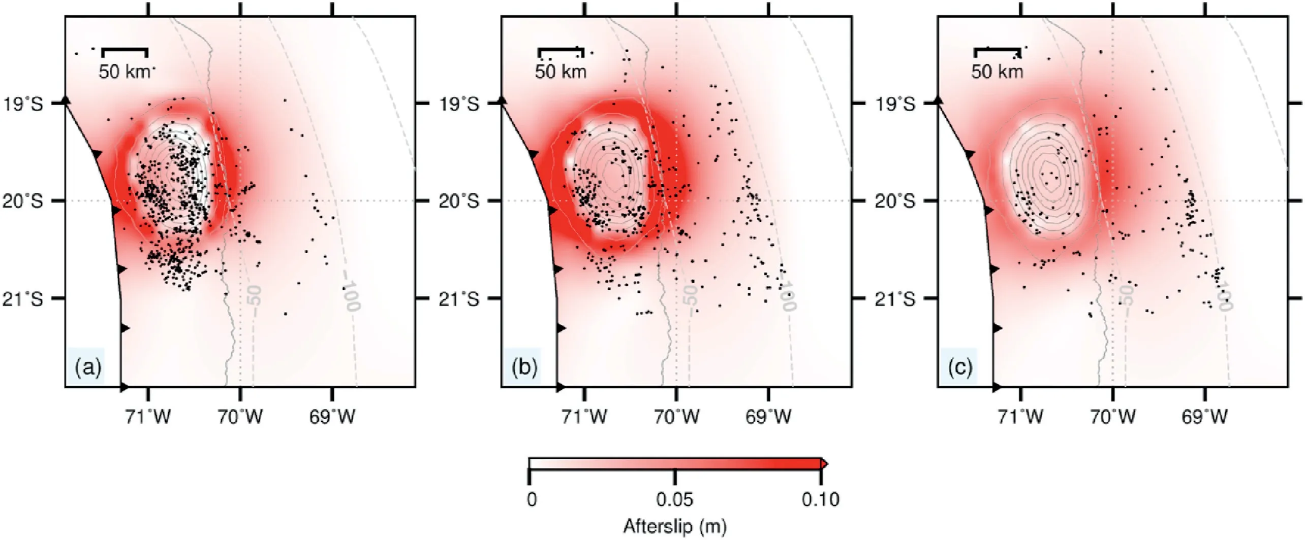
Fig.7.Distribution and evolution of the afterslip.Colored contours represent the afterslip.Gray solid contour lines represent the coseismic slip of the 2014 Iquique earthquake (Schurr et al.,2014).Black dots represent aftershocks near the subduction surface in each phase.(a) Cumulative afterslip within the first month after the 2014 Iquique earthquake.(b) Cumulative afterslip in the 2-6 months after the 2014 Iquique earthquake.(c) Cumulative afterslip in the 6-12 months after the 2014 Iquique earthquake.(For interpretation of the references to color in this figure legend,the reader is referred to the Web version of this article.)

4.Discussion

Different geophysical studies on subduction zones have shown that there is a thin weak layer underlying the oceanic lithosphere.For example,Naif et al.(2013) reported a high-conductivity layer at the depths of 45-70 km at the middle America trench beneath the subducting Cocos plate(～23 Ma)through analyzing sea-floor magnetotelluric data.Stern et al.(2015) obtained a thin channel underlying the 120-Ma oceanic plate beneath the North Island of New Zealand through seismic reflection imaging.

The Southern-Peru northern-Chile subduction zone is an ideal place to investigate the interaction between a subducting slab and the surrounding mantle.Scire et al.(2015)used teleseismic P-wave tomography to image velocity anomalies in the mantle between 18°and 28°S.Their model well resolved a low-velocity anomaly layer below the subducting slab at depths between 150 and 300 km depth.This is consistent with the asthenospheric properties obtained in this work.The order of the asthenospheric viscosity in this work is also consistent with that in Hu et al.(2016b).

Our model fits the first-order pattern of the observed post-seismic displacements.The worse fit to a few coastal stations,a similar magnitude but about 30°off the direction comparing to the observations,may be due to higher order of heterogeneities in the afterslip that is not considered in this work.In addition,possible poroelastic response and along-strike slab interface geometry also complicate the efforts to obtain a better fit to the observations of those coastal stations.

Global studies on the rheological properties of the upper mantle,such as simulating the subduction history and the dynamic processes of the oceanic asthenosphere(Liu and Stegman,2011;Liu and Zhou,2015)and glacial isostatic adjustment(e.g.Peltier et al.,2015),reported viscosities of the mantle wedge to be one to three orders of magnitude higher than that in this work.This is likely due to the following reasons.Firstly,the global studies may present constraints on the overall rheological properties of the upper mantle.However,in this work we focused only on the subduction zone.Secondly,the dehydration process of the subduction slab may weaken the localized over-riding mantle wedge and thus lead to a lower viscosity in the mantle wedge.Finally,the deformation time scale may also play an important role in determining the effective viscosity of the mantle wedge.The fast earthquake cycle deformation considered in this work certainly dictates a greater amount of the strain-rate-weakening comparing to more sluggish mantle convection rate.

5.Conclusions

In this study we developed a 3D viscoelastic finite model to study the post-seismic deformation of the 2014MW8.1 Iquique earthquake and obtained the first-order rheological structure of the northern Chile-southern Peru subduction zone.We carried out systematic tests on the viscosity of the shear zone,depth and viscosity of asthenosphere.We evaluated 150 test models through comparing observed postseismic displacements with model predictions.We obtained our lowest misfit model via the grid search.The viscosity of the shear zone,depth and viscosity of the oceanic asthenosphere in the lowest misfit model are determined to be 1017Pa s,110 km and 2×1018Pa s,respectively.These obtained values are consistent with previous studies on other subduction zones,such as Cascadia(Wang et al.,2012),NE Japan(Hu et al.,2016b;Sun et al.,2018),Alaska(Suito and Freymueller,2009)and Sumatra(Hu et al.,2012).

We studied the individual contribution of the rheological units to the postseismic crustal deformation.The main features are as follows.The seaward motion is controlled mainly by the afterslip and the viscoelastic relaxation in the mantle wedge.Subsidence near the rupture area offshore is controlled mainly by the viscoelastic relaxation in the asthenosphere that also causes the landward motion.There are tradeoffs among the rheological units,for example,a good fit to the vertical component near the trench requires a low viscosity in the asthenosphere but causes smaller horizontal displacements.

We applied a 2 km thick weak shear zone attached to the fault to simulate the stress-driven,time-dependent afterslip surrounding the rupture area.The viscosity of the shear zone is determined to be 1017Pa s,on the same order of that in NE Japan(Hu et al.,2016a).The result of our model shows that accumulated afterslip within 1 year after the event is up to～40 cm.It decreases rapidly with time and becomes negligibly small after 2 years since the event.The estimate of our model is smaller than that of Hoffmann et al.(2018)because our model considers the viscoelastic response to time-dependent afterslip which may represent a more real postseismic process.

Acknowledgement

We thank the editor and two anonymous reviewers for the comments to improve the manuscript.This work was supported by the National Key R&D Program(2018YFC504103).Strategic Priority Research Program of Chinese Academy of Sciences(XDA20070302),and the National Natural Science Foundation of China(41774109).The numerical calculations in this paper have been done on the supercomputing system in the Supercomputing Center of University of Science and Technology of China.