EXISTENCE THEOREM FOR A CLASS OF MEMS MODEL WITH A PERTURBATION TERM

LV Jia-qi ， CHEN Nan-bo ， LIU Xiao-chun

(1. School of Mathematics and Statistics， Wuhan University， Wuhan 430072， China)(2. School of Mathematics and Computing Science， Guilin University of Electronic Technology，Guilin 541004， China)

Abstract: In this paper， we study a class of MEMS models with a perturbation term. With the help of upper and lower solution method and variational approach， we obtain the existence and multiplicity results for these models. In particular， we find a curve which splits the area of parameters in the first quadrant into two parts according to the existence of solutions for a MEMS system. These are an extension on the existing literature in the aspect of MEMS models.

Keywords: MEMS model; a perturbation term; variational method; upper and lower solution

1 Introduction

In this paper we discuss the existence and nonexistence of solutions to the following MEMS equation

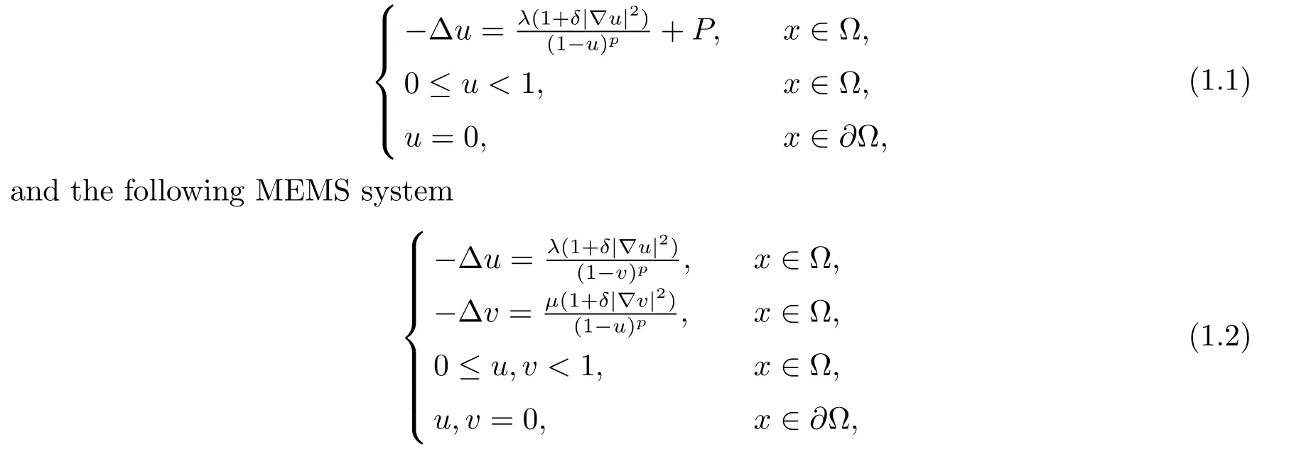
where Ω is a bounded domain in RNwithN ≥3，p ＞1 andλ，μ，δ，Pare all positive parameters. The relevant problems corresponding to(1.1)，(1.2)have been studied in various areas such as mathematics， physics and so forth.

In fact， problems like equation (1.1) originally came from the so-called MEMS model which MEMS means Micro-Electro-Mechanical Systems. This model describes the motion of an elastic membrane supported on a fixed ground plate and has been extensively studied for decades. Here we quote some of them and more details can be found in [1-8] and references therein.

MEMS device is composed of an elastic membrane supported on a fixed ground plate.When a voltageλis applied， the elastic membrane deflects toward the ground plate. While the voltage exceeds a critical valueλ*， the two plates touch and no longer separate. This state is called unstable. MEMS device is no longer working properly. However， for the sake of research convenience， most researchers regard the parallel plates as infinite in length and ignore electrostatic field at the edges of the plates. After approximation， the authors in papers [6-8] introduced the following model

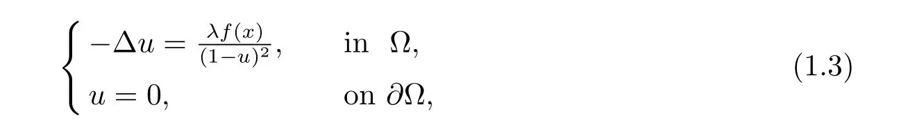
where Ω⊂RNis a bounded domain andf(x)∈C(Ω) is a non-negative function. In [6]， the authors applied analytical and numerical techniques to establish upper and lower bounds forλ*which is a critical value of (1.3). They also obtained some properties of the stable and semistable solution such as regularity，uniqueness， multiplicity and so on. In[7]， the authors proved the existence of the second solution by variational approach and got the compactness along the branches of unstable solution. In [8]， the authors applied the extend Pohozaev identity and addressed that whenλis a small voltage and the domain Ω is bounded and star-shaped， then stable solution is the unique solution.

In[9]， Cassani，Marcos and Ghoussoub investigated the existence of biharmonic type as follows:

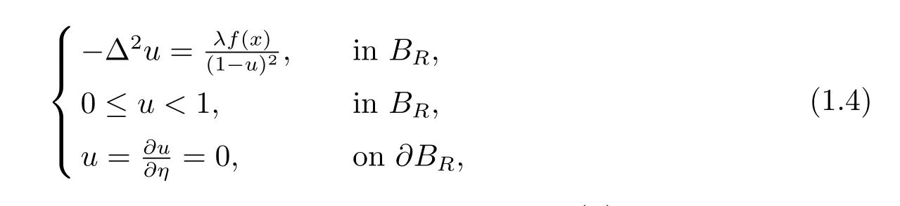
whereBRis a ball in RNcentered at the origin with radiusR， 0≤f(x)≤1 andηdenotes the unit outward normal to∂BR. They proved that， there exists aλ*=λ*(R，f)＞0 such that for 0＜λ ＜λ*， problem (1.4) possesses a minimal positive and stable solutionuλ.

Since the approximation of (1.3) brings some errors in some cases， the models (1.3)need be corrected in several manners. In [10， 11]， the authors started to consider the effect of edges of plates and added the corner-corrected term in (1.3). For instance， the authors in[11] studied the following equation

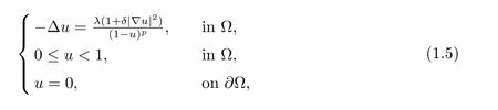
whereδ ＞0，p ＞1 andλ ＞0. They obtained the existence and nonexistence result depending onδand someλ*δ ＞0.

If we correct the model (1.3) with external force or pressure， it can be reduced to

whereP ＞0 is a parameter. In [12]， Guo， Zhang and Zhou obtained the existence and nonexistence result of (1.6) which depends onλandP.

Inspired by the researches in [11-13]， we will study the problem (1.1) and get our first result.

Theorem 1.1 For anyδ ＞0， we have

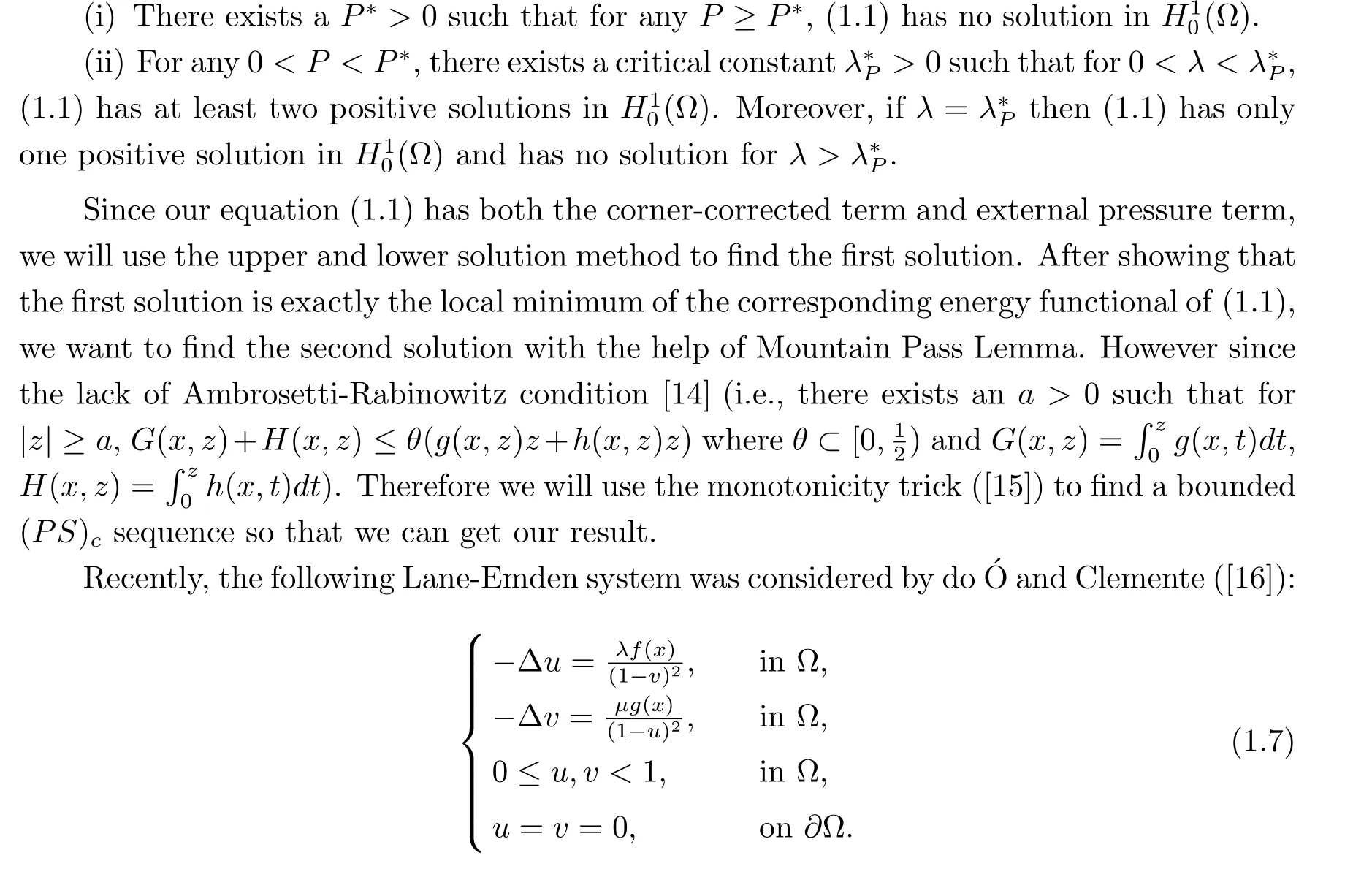
They obtained a curve Γ that separates the positive quadrant of the (λ，μ)-plane into two connected componentsO1andO2. For (λ，μ)∈O1， problem (1.7) has a positive classical minimal solution (uλ，vλ). If (λ，μ)∈O2， there is no solution.

Motivated by the result in [16]， we consider the system (1.2) in the second part. With the help of upper and lower solution approach we get the next result.

Theorem 1.2 There exists a curve Γ which splits the parameter area (λ，μ) of the first quadrant into two connected partsD1andD2. When (λ，μ)∈D1， (1.2) has at least one solution. There is no solution if (λ，μ)∈D2.

The rest of our paper is organized as follows. In Section 2， we will introduce a function transformation to(1.1)and some auxilary results. In Section 3，we give the proof of Theorem 1.1. In Section 4， we show the proof of Theorem 1.2.

2 Preliminaries

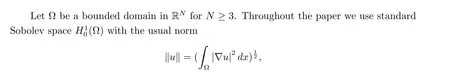
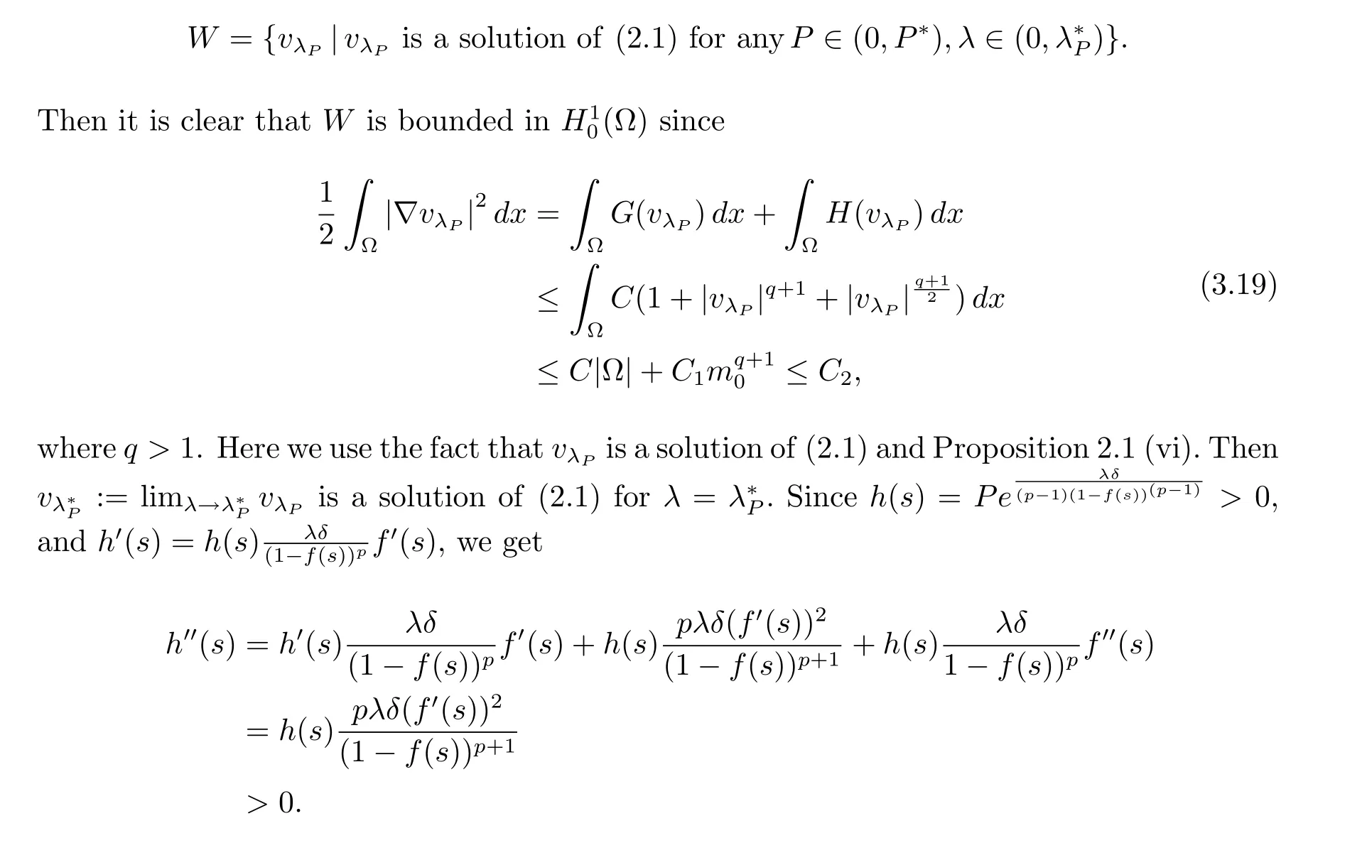
and the usual Lebesgue spaceLp(Ω) whose norms are denoted by|u|p. Since it is hard to write the concrete form of energy functional of (1.1)，we introduce a function transformation to overcome this difficulty. Set

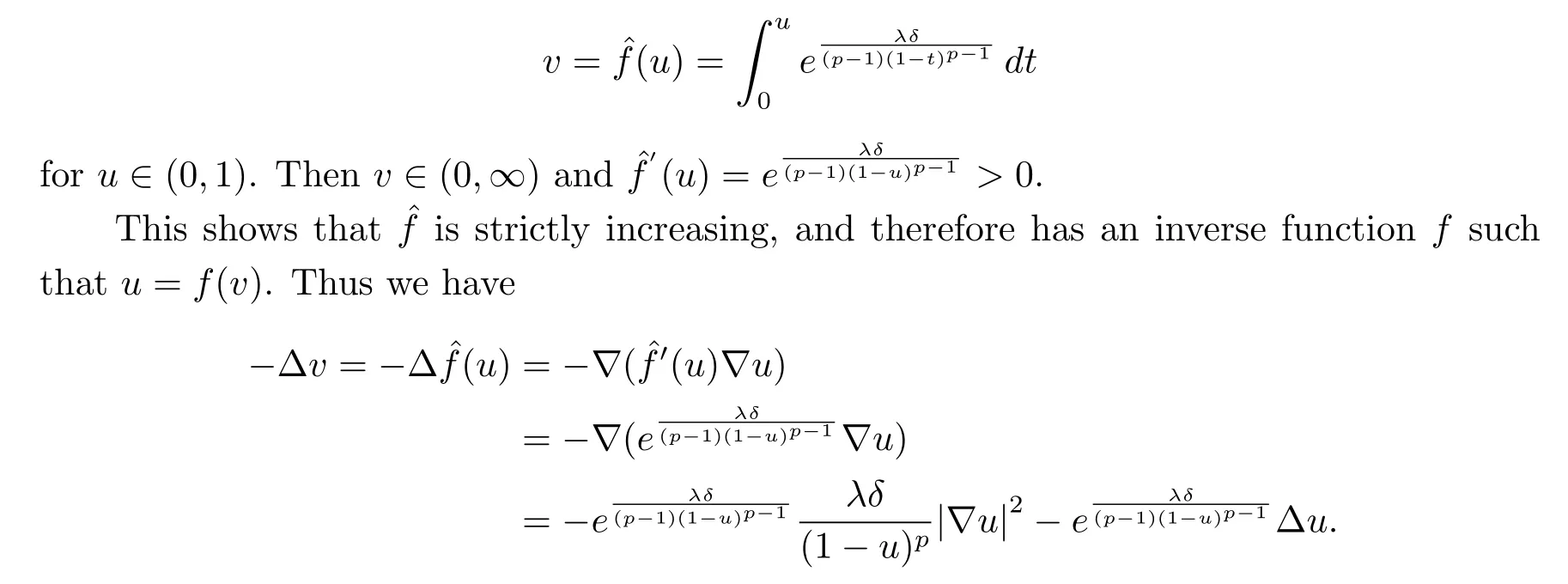
Together with (1.1)， we know that the existence of solution to (1.1) is equivalent to the existence of the following equation

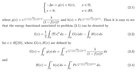
We will give some properties satisfied byg(s)，h(s) andG(s)，H(s) defined by (2.1)，(2.3) and (2.4). In the sequel，C，C′，C′′，Ci(i ∈N+) represent different constants in the different circumstances.

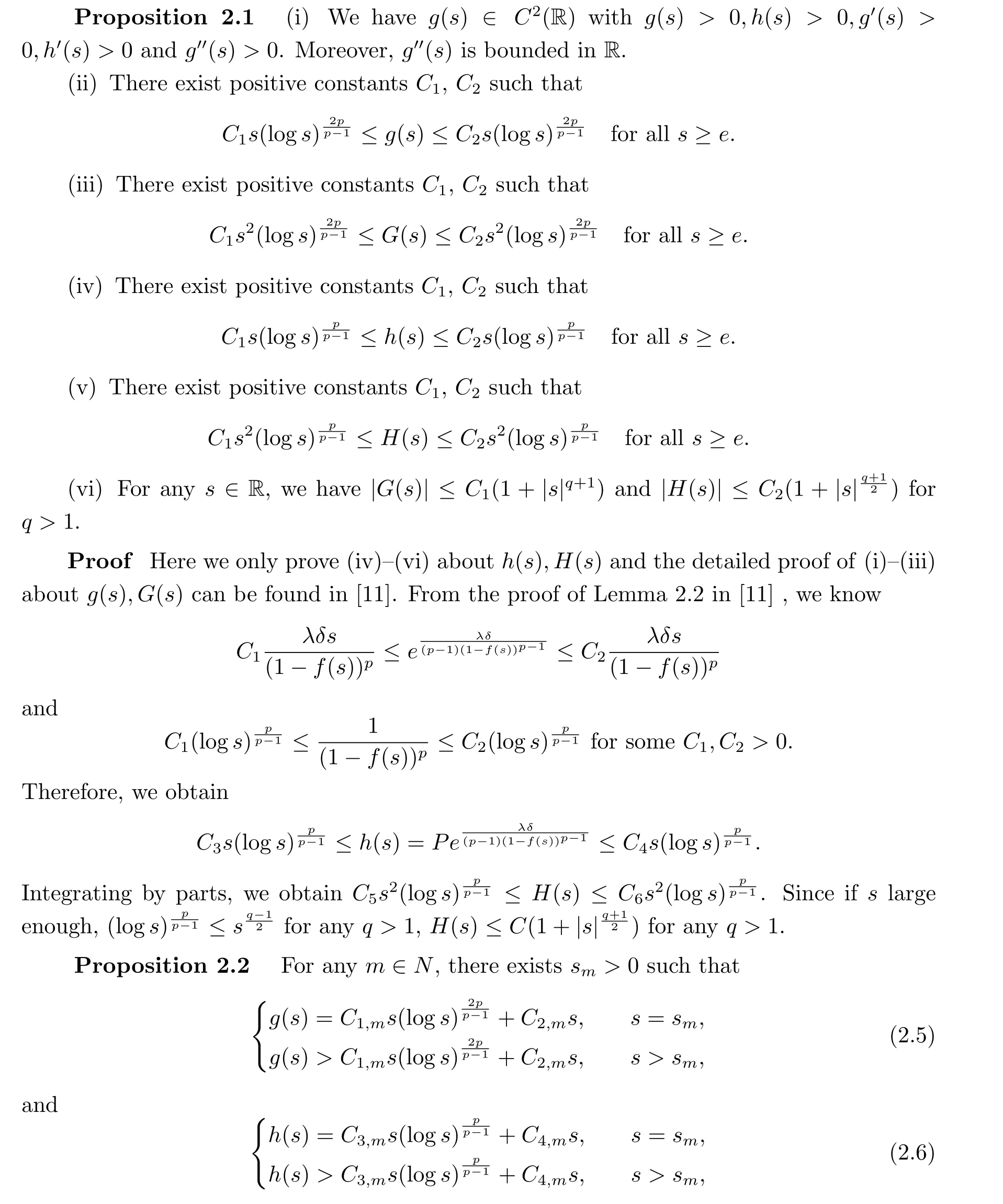
whereCi，m ＞0 (i=1，2，3，4) are positive constants depending onm.

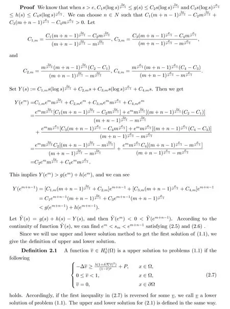
We will use the variational method to find the second solution of (1.1)， and therefore we recall some basic results about this method.

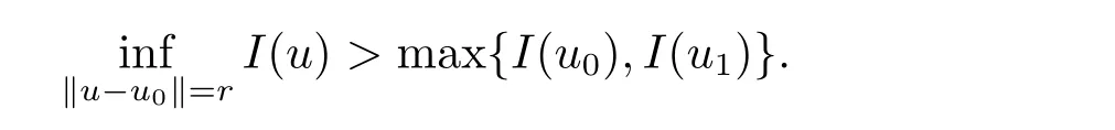
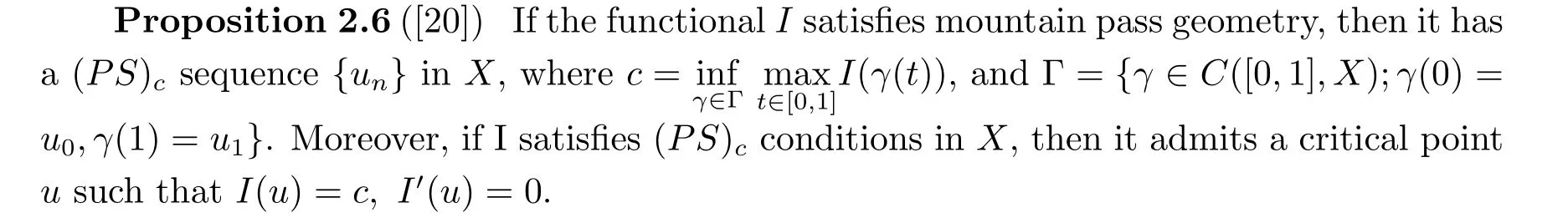
Definition 2.2 ([20]) Given a real Banach spaceX， we say a functionalI:X →R of classC1satisfying the mountain pass geometry if there existsu0，u1∈Xand 0＜r ＜‖u1-u0‖such that

We define the Palais-Smale sequence at levelc((PS)csequence for short) and (PS)cconditions inXforIas follows.

Definition 2.3

(i) Forc ∈R， a sequence{un}is a (PS)csequence inXforIifI(un)→c，I′(un)→0 asn →∞.

(ii)Isatisfies the (PS)ccondition inXif every (PS)csequence inXforIcontains a convergent subsequence.

Now we quote the Mountain Pass Lemma.

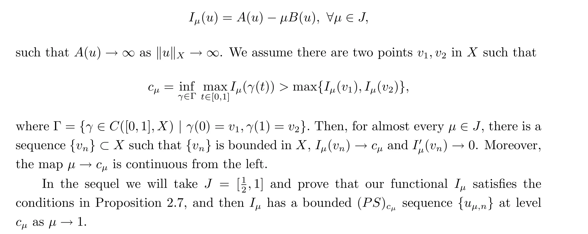
In order to find a bounded (PS)csequence for the functionalIinH10(Ω)， we recall the following monotonicity trick.

Proposition 2.7 ([21]) LetXbe a Banach space equipped with a norm‖·‖XandJ ⊂R+be an interval. We consider a family{Iμ}μ∈JofC1-functionals onXof the form

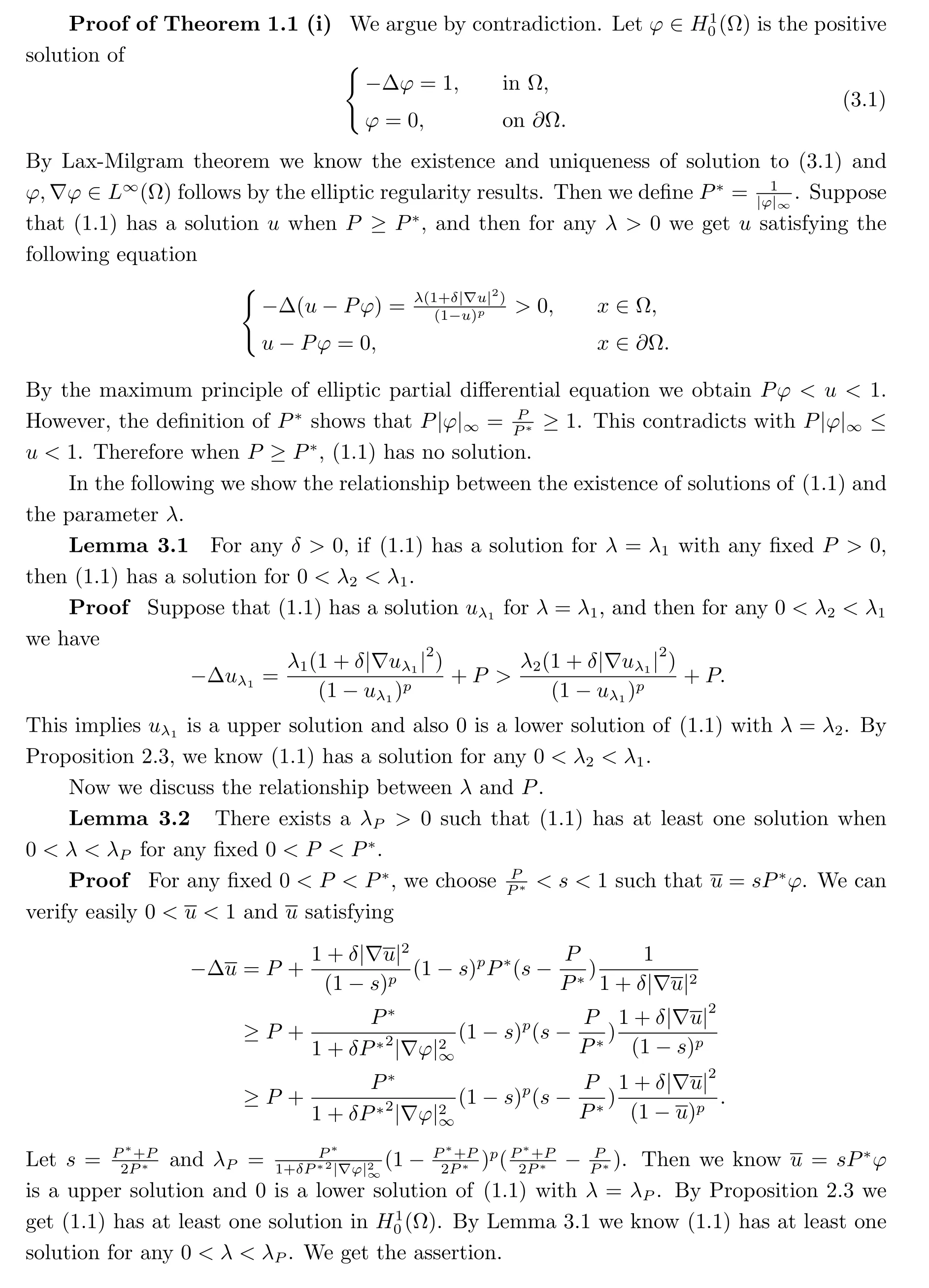
3 The proof of Theorem 1.1

In this section，we will give the proof of Theorem 1.1. First we will show the nonexistence result for (1.1).

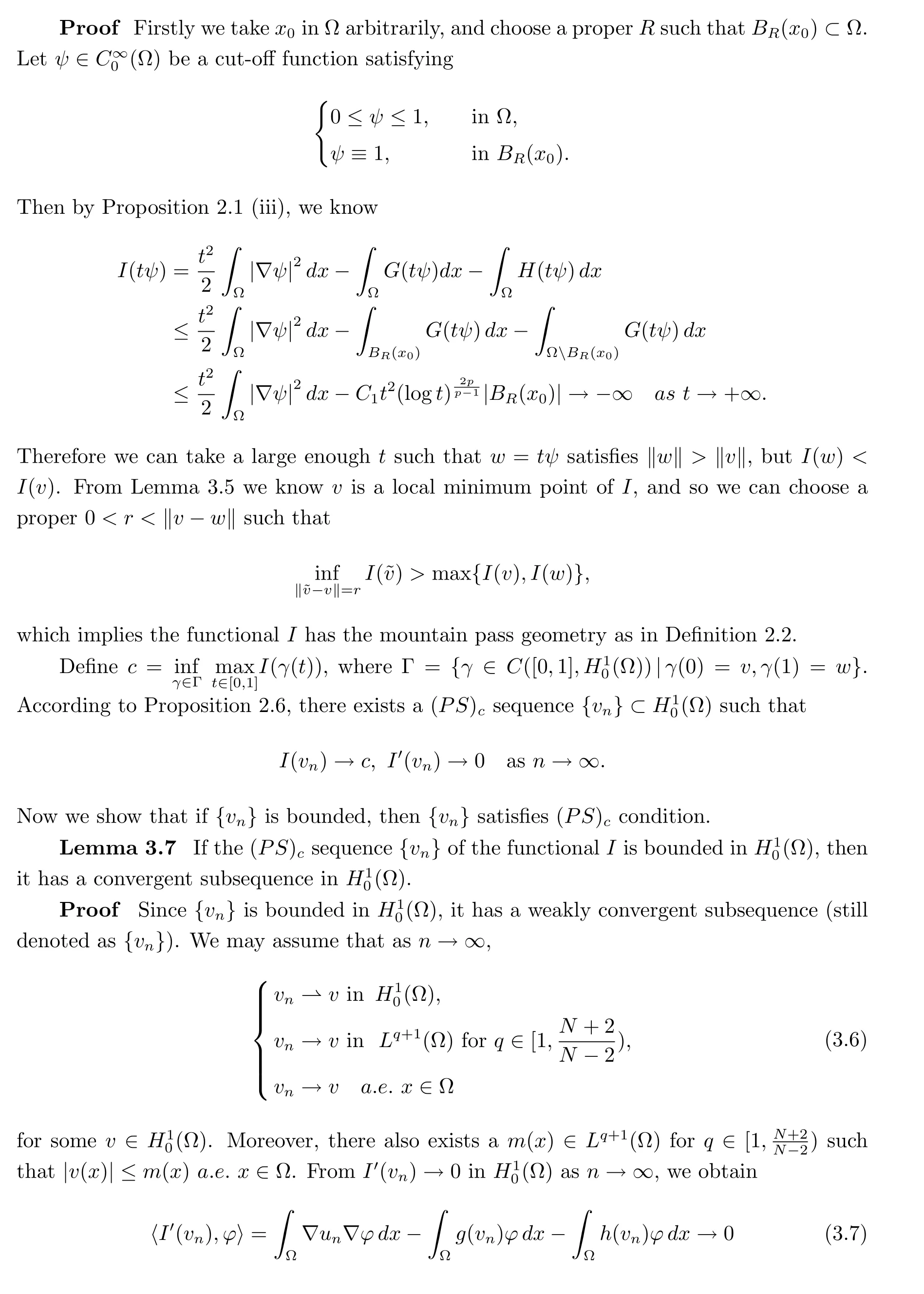
Lemma 3.6 The energy functionalIin (2.2) has a mountain pass geometry.

4 The proof of Theorem 1.2

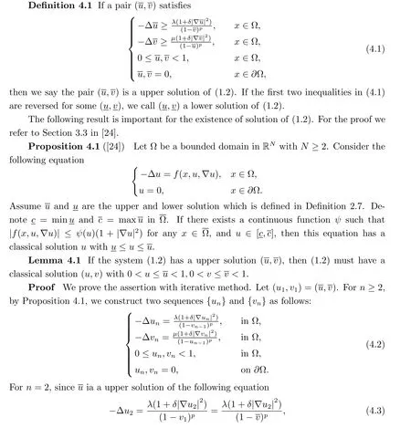
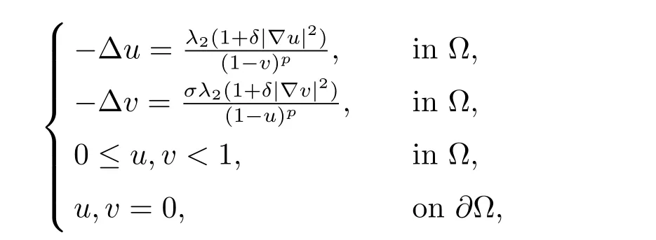
In this section， we focus on the equation (1.2)， i.e.，

whereλ，μ，δare positive parameters andp ＞1.It is interesting to find that the existence of solution of (1.2) depends on the parameter area (λ，μ) in the first quadrant. We will again apply the upper and lower solution method to get the proof of Theorem 1.2.

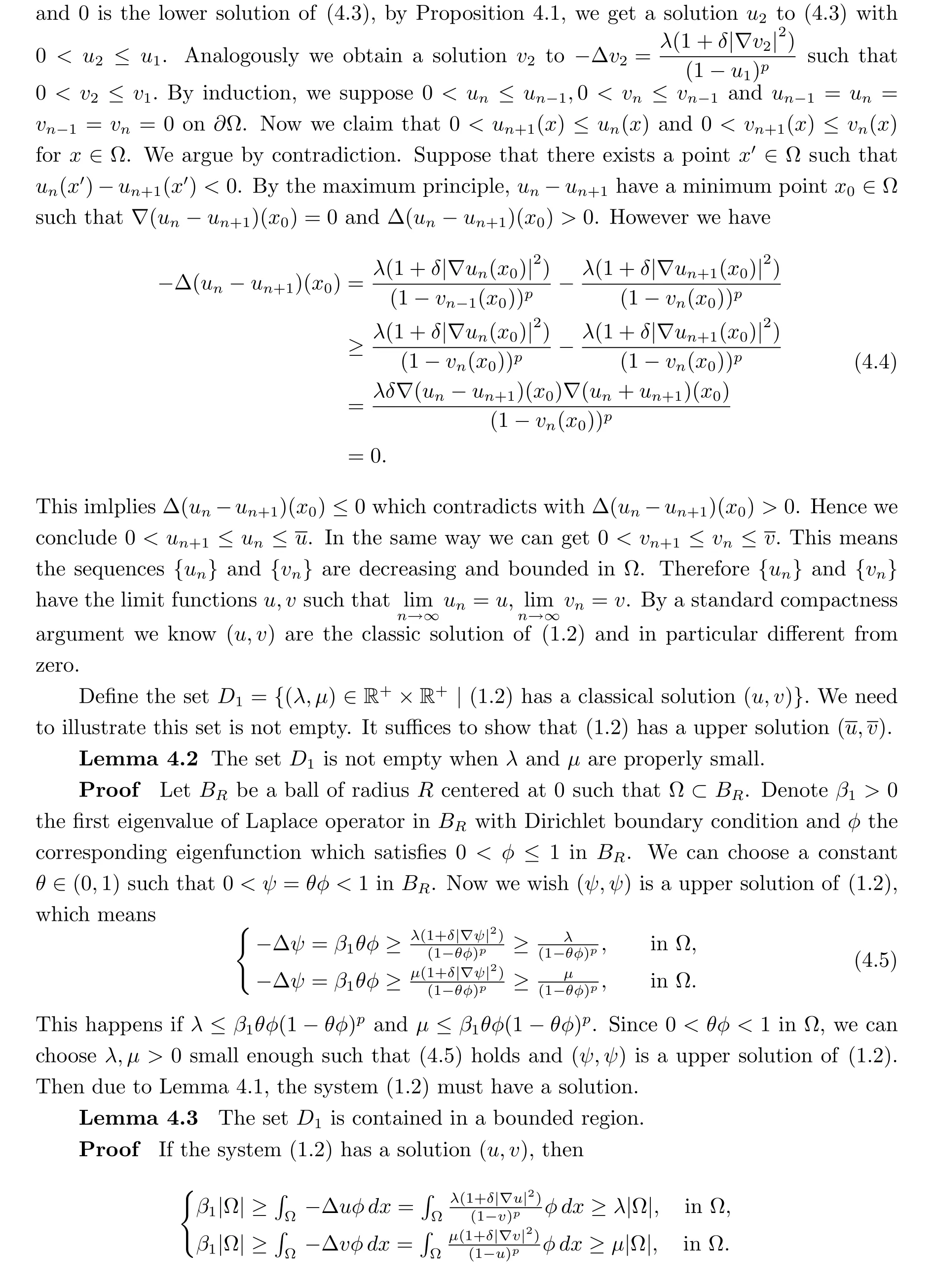
This impliesλ ≤β1andμ ≤β1. HenceD1⊂(0，β1]×(0，β1] is bounded.

Lemma 4.4 If the system (1.2) has a solution with the parameter pair (λ，μ)∈D1，then (λ′，μ′) is still inD1for anyλ′≤λ，μ′≤μ.

Proof It is easy to verify that the solution (u，v) with the parameter pair (λ，μ) is a upper solution of the system (1.2) with the pair (λ′，μ′). Then by Lemma 4.1 we know the system (1.2) must have at least one solution.

Based on the above-mentioned argument， we can find a curve Γ in the first quadrant of (λ，μ)-plane such that the existence of (1.2) depends on the region divided by Γ. More precisely， for anyσ ＞0， we define

It is obvious that{(λ，σλ)∈R+×R+| 0＜λ ≤λ*(σ)}⊂D1and{(λ，σλ)∈R+×R+|λ ＞λ*(σ)}∩D1=∅. We also can defineμ*(σ)=σλ*(σ).

Lemma 4.5 The curve Γ(σ)=(λ*(σ)，μ*(σ)) is continuous.

Proof We prove this by contradiction. Suppose that Γ(σ) is not continuous at someσ0＞0. Then there existsε0＞0 such that for anyη ＞0， when 0＜|σ-σ0|＜ηwe have|Γ(σ)-Γ(σ0)|＞ε0.This implies either the caseλ*(σ)＞λ*(σ0)，μ*(σ)＞μ*(σ0) or the caseλ*(σ)＜λ*(σ0)，μ*(σ)＜μ*(σ0) appears. Without loss of generality， we just discuss the first case. Letλ1，λ2＞0 such thatλ*(σ)＞λ2＞λ1＞λ*(σ0)，μ*(σ)＞σλ2＞σ0λ1＞μ*(σ0). By the definition ofλ*(σ)， we obtain

then we have a solution (uλ2，vλ2). Obviously it is a upper solution of the system (1.2) when parameter pair equals to (λ1，σ0λ1).This impliesλ1≤λ*(σ0) which contradicts with the assumptionλ1＞λ*(σ0).

Lemma 4.6λ*(σ) is decreasing andμ*(σ) is increasing with respect toσ.

Proof (i)We first show thatλ*(σ)is decreasing. We argue by contradiction. Suppose thatλ*(σ1)＜λ*(σ2) forσ1＜σ2. Thenμ*(σ1) =σ1λ*(σ1)＜σ2λ*(σ2) =μ*(σ2). We can choose two constantsλ1，λ2such thatλ*(σ1)＜λ1＜λ2＜λ*(σ2) andσ1λ*(σ1)＜σ1λ1＜σ2λ2＜σ2λ*(σ2). Similar to the proof process as in Lemma 4.5， we can obtainλ*(σ1)≥λ1which is contradicted withλ*(σ1)＜λ1. Hence the hypothesis is not valid andλ*(σ) is decreasing.

(ii) We next show thatμ*(σ) is increasing. We argue again by contradiction. Suppose thatμ*(σ1) =σ1λ*(σ1)＞μ*(σ2) =σ2λ*(σ2) forσ1＜σ2. By (i)， we knowλ*(σ1)＞λ*(σ2).Therefore we can choose two proper constantsλ1，λ2＞0 such thatλ*(σ1)＞λ1＞λ2＞λ*(σ2) andσ1λ*(σ1)＞σ2λ1＞σ2λ2＞σ2λ*(σ2). By Lemma 4.4， we conclude the system(1.2) has one solution with parameter pair (λ2，σ2λ2). This impliesλ2≤λ*(σ2) which contradicts withλ2＞λ*(σ2). We finish the proof.

Now we can give the proof of Theorem 1.2.

Proof of Theorem 1.2 By Lemma 4.2，4.3，4.5 and 4.6，if we takeμ*(σ)as horizontal axis andλ*(σ)as vertical axis，then the curve Γ(σ)=(λ*(σ)，μ*(σ))splits the first quadrant of (μ*(σ)，λ*(σ))-plane into two connected parts. When the parameter pair is above the curve Γ， there is no solution of (1.2). While the parameter pair is below the curve， there exists at least one solution of (1.2).